4 Dynamic Programming
4.1 Policy Evaluation
The Bellman equations for state-value Equation 3.12 and for action-value Equation 3.13 can be used as update rules to approximate \(v_\pi\) and \(q_\pi\): \[ v_{k+1}(s) = \sum_a \pi(a|s) \sum_{s',r} p(s',r|s,a)[r+\gamma v_{k}(s')] \tag{4.1}\] \[ q_{k+1}(s,a) = \sum_{s',r}p(s',r|s,a) [r + \gamma \sum_{a'}\pi(a'|s')q_k(s',a')] \tag{4.2}\]
These equations form the basis for iterative policy evaluation. The algorithm below demonstrates how to approximate \(v_\pi\), where updates are performed in “sweeps” rather than “chunk updates”. This constitutes the policy evaluations step,\(\pi \overset{\mathrm{Eval}}{\to} v_{\pi}\), in the policy iteration algorithm (Section 4.3).
Input: \(\pi\), the policy to be evaluated
Parameters: \(\theta > 0\), determining accuracy of estimation
Initialisation: \(V(s)\), for all \(s \in \mathcal{S}\) arbitrarily, and \(V(\mathrm{terminal}) = 0\)
Loop:
\(\Delta \gets 0\)
Loop for each \(s \in \mathcal{S}\):
\(v \gets V(s)\)
\(V(s) \gets \sum_a \pi(a|s) \sum_{s',r}p(s',r|s,a)[r + \gamma V(s')]\)
\(\Delta \gets \max(\Delta, |v - V(s))\)
until \(\Delta < \theta\)
Example 4.1 Here we explore Example 4.1 from Sutton and Barto (2018)
Here is the quick summary:
- states: non-terminal states are numbered 1 through 14. The two gray cells are treated as a single terminal state.
- actions: Four deterministic actions available in each state: up, down, left, right. Moving “off the grid” results in no state change.
- rewards: A reward of -1 is given for every transition until the terminal state is reached
- return: undiscounted
And here are the state-values for the random policy:
Note that these values are (luckily) exact, which will be useful for the next exercises
Exercise 4.1 In Example 4.1, if \(\pi\) is the equiprobable random policy, what is \(q_\pi(11, \mathrm{down})\)? What is \(q_\pi(7, \mathrm{down})\)?
Solution 4.1. We can use the state-value function given in the example: \[ \begin{split} q_\pi(11, \mathrm{down}) &= -1 + 0 = -1\\ q_\pi(7, \mathrm{down}) &= -1 + v_\pi(11) = -1 + (-14) = -15 \end{split} \]
Exercise 4.2 In Example 4.1, suppose a new state 15 is added to the gridworld just below state 13, and its actions, left, up, right, and down, take the agent to states 12, 13, 14, and 15, respectively. Assume that the transitions from the original states are unchanged. What, then, is \(v_\pi(15)\) for the equiprobable random policy?
Now suppose the dynamics of state 13 are also changed, such that action down from state 13 takes the agent to the new state 15. What is \(v_\pi(15)\) for the equiprobable random policy in this case?
Solution 4.2. Since the MDP is deterministic and all transitions give the same reward, the undiscounted Bellman equation Equation 3.12 simplifies to: \[ v_{\pi}(s) = r + \sum_{a}\pi(a|s') [v_{\pi}(s')], \]
where \(r = -1\).
The first case is quite easy to compute. The transitions for all original states remain unchanged, so their values also remain unchanged. For the new state 15, we can write: \[ v_\pi(15) = -1 + \frac{1}{4}(v_\pi(12) + v_\pi(13) + v_\pi(14) + v_\pi(15)) \] which gives \(v_\pi(15) = -20\).
Now in the second case we might be up for a lot of work, as state 13 has a new transition: taking action “down” leads to state 15. This changes the dynamics of the MDP, so in principle the values might change. However, luckily the existing state-value function still satisfies the Bellman equation for state 13: \[ v_\pi(13) = -1 + \frac{1}{4}(v_\pi(12) + v_\pi(9) + v_\pi(13) + v_\pi(15)) \]
Substitute the known values we see that the equation holds \[ v_\pi(13) = -20 = -1 + \frac{1}{4}(-22 - 20 - 14 - 20) \]
So \(v_\pi(13)\) remains consistent with the new dynamics. Since all Bellman equations continue to hold with the same values, the state-value function does not change. So, \(v_\pi(15)=-20\) also in this case.
Exercise 4.3 What are the equations analogous to Equation 3.10, Equation 3.12, and Equation 4.1 for the action-value function \(q_\pi\) and its successive approximation by a sequence of functions \(q_0, q_1, \dots\)?
Solution 4.3. We have already stated these equations in tandem as Equation 3.11, Equation 3.13, and Equation 4.2.
4.2 Policy Improvement
An optimal policy can always be chosen to be deterministic. This is quite intuitive: why would introducing randomness in action selection be beneficial if all you care about is maximising expected return? More rigorously, if you are choosing between two actions, \(a_1\) and \(a_2\), and you know their values \(q_\pi(s,a_1)\) and \(q_\pi(s,a_2)\), then it is clearly best to take the one with the higher value. A key tool for this kind of reasoning is the policy improvement theorem.
Theorem 4.1 Let \(\pi\) be any policy and \(\pi'\) a deterministic policy. Then \(\pi \leq \pi'\) if \[ v_\pi(s) \leq q_\pi(s,\pi'(s)), \] for all \(s \in \mathcal{S}\).
Proof. From the assumption, we have: \[ \begin{split} v_\pi(s) &\leq q_\pi(s, \pi'(s)) \\ &= \mathbb{E}[R_{t+1} + \gamma v_\pi(S_{t+1}) \mid S_t = s, A_t = \pi'(s)] \\ &= \mathbb{E}_{\pi'}[R_{t+1} + \gamma v_\pi(S_{t+1}) \mid S_t = s] \\ \end{split} \] (if you wonder about the indices in the expectation: the first expectation is completely determined by the MDP, in the second one we stipulate action selection according to \(\pi'\).)
Now, we can unroll this expression recursively: \[ \begin{align} v_\pi(s) &\leq \mathbb{E}_{\pi'}[R_{t+1} + \gamma v_\pi(S_{t+1}) \mid S_t = s] \\ &\leq \mathbb{E}_{\pi'}[R_{t+1} + \gamma \mathbb{E}_{\pi'}[R'_{t+2} + \gamma v_\pi(S'_{t+2}) \mid S'_{t+1} = S_{t+1}] \mid S_t = s] \\ &= \mathbb{E}_{\pi'}[R_{t+1} + \gamma R_{t+2} + \gamma^2 v_\pi(S_{t+2}) \mid S_t = s] \end{align} \]
and so on. The last equality should be justified formally by the law of total expectation and the law of the unconscious statistician (Theorem 2.4 and Theorem 2.1).
Iterating this process a couple of times we get \[ v_\pi(s) \leq \mathbb{E}_{\pi'}\bigg[\sum_{i=0}^{N} \gamma^i R_{t+1+i} + \gamma^{N+1} v_\pi(S_{t+1+N}) \;\bigg|\; S_t = s \bigg] \]
and in the limit (everything is bounded so this should be kosher) \[ v_\pi(s) \leq \mathbb{E}_{\pi'}\bigg[\sum_{i=0}^{\infty} \gamma^i R_{t+1+i} \;\bigg| \; S_t = s \bigg] = v_{\pi'}(s). \]
This result allows us to show that every finite MDP has an optimal deterministic policy.
Let \(\pi\) be any policy. Define a new deterministic policy \(\pi'\) by \[ \pi'(s)= \underset{a \in \mathcal{A}}{\mathrm{argmax}} q_{\pi}(s,a) \]
By the policy improvement theorem, we have \(\pi \leq \pi'\). Now consider two deterministic policies, \(\pi_1\) and \(\pi_2\), and define their meet (pointwise maximum policy) as \[ (\pi_1 \vee \pi_2)(s) = \begin{cases}\pi_1(s) &\text{if } v_{\pi_1}(s) \geq v_{\pi_2}(s) \\ \pi_2(s) &\text{else} \end{cases} \]
Then, again by the policy improvement theorem, we have \(\pi_1, \pi_2 \leq \pi_1 \vee \pi_2\).
Now, since the number of deterministic policies is finite (as both \(\mathcal{S}\) and \(\mathcal{A}\) are finite), we can take the meet over all deterministic policies and obtain an optimal deterministic policy.
This leads directly to a characterisation of optimality in terms of greedy action selection.
Theorem 4.2 A policy \(\pi\) is optimal, if and only if, \[ v_\pi(s) = \max_{a \in \mathcal{A}(s)} q_{\pi}(s,a), \tag{4.3}\]
for all \(s \in \mathcal{S}\).
Proof. If \(\pi\) is optimal then \(v_\pi(s) < \max_{a} q_\pi(s,a)\) would lead to a contradiction using the policy improvement theorem.
For the converse we do an argument very similar to the proof of Theorem 4.1. So similar in fact that I’m afraid that were doing the same work twice. Let \(\pi\) satisfy Equation 4.3. We show that \(\pi\) is optimal by showing that \[ \Delta(s) = v_{\pi_*}(s) - v_{\pi}(s) \] is \(0\) for all \(s \in \mathcal{S}\), where \(\pi_*\) is any deterministic, optimal policy.
We can bound \(\Delta(s)\) like so \[ \begin{split} \Delta(s) &= q_{\pi_*}(s,\pi_*(s)) - \max_a q_{\pi}(s,a) \\ &\leq q_{\pi_*}(s,\pi_*(s)) - q_\pi(s,\pi_*(s)) \\ &= \mathbb{E}_{\pi_*}[ R_{t+1} + \gamma v_{\pi_*}(S_{t+1}) - (R_{t+1} + \gamma v_{\pi}(S_{t+1})) | S_{t} = s] \\ &= \mathbb{E}_{\pi_*}[\gamma \Delta(S_{t+1}) | S_t = s] \end{split} \]
Iterating this and taking the limit gives \[ \Delta(s) \leq \lim_{k \to \infty} \mathbb{E}_{\pi_*}[\gamma^k \Delta(S_{t+k}) \mid S_t = s] = 0. \]
For a policy \(\pi\), if we define \(\pi'(s) := \underset{a}{\mathrm{argmax}}\;q_\pi(s,a)\), we get an improved policy, unless \(\pi\) was already optimal. This constitutes the policy improvement step,\(v_\pi \overset{\mathrm{Imp}}{\to} \pi'\), in the policy iteration algorithm.
4.3 Policy Iteration
The policy iteration algorithm chains evaluation and improvement and converges to an optimal policy, for any initial policy \(\pi_0\): \[ \pi_0 \overset{\mathrm{Eval}}{\to} v_{\pi_0} \overset{\mathrm{Imp}}{\to} \pi_1 \overset{\mathrm{Eval}}{\to} v_{\pi_1} \overset{\mathrm{Imp}}{\to} \pi_2 \overset{\mathrm{Eval}}{\to} v_{\pi_2} \overset{\mathrm{Imp}}{\to} \dots \overset{\mathrm{Imp}}{\to} \pi_* \overset{\mathrm{Eval}}{\to} v_{*} \]
And here is the pseudo code.
Parameter:
\(\theta\): a small positive number determining the accuracy of estimation
1. Initialisation:
\(V(s) \in \mathbb{R}\), \(\pi(s) \in \mathcal{A}(s)\) arbitrarily, \(V(\mathrm{terminal}) = 0\)
2. Policy Evaluation
Loop:
\(\Delta \gets 0\)
Loop for each \(s \in \mathcal{S}\):
\(v \gets V(s)\)
\(V(s) \gets \sum_{s',r}p(s',r|s,\pi(s))[r + \gamma V(s')]\)
\(\Delta \gets \max(\Delta, |v - V(s)|)\)
until \(\Delta < \theta\)
3. Policy Improvement
\(\text{policy-stable} \gets \mathrm{true}\)
For each \(s \in \mathcal{S}\):
\(\text{old-action} \gets \pi(s)\)
\(\pi(s) \gets \underset{a}{\mathrm{argmax}} \sum_{s',r} p(s', r |s,a)[r + \gamma V(s')]\)
If \(\text{old-action} \neq \pi(s)\), then \(\text{policy-stable} \gets \text{false}\)
If \(\text{policy-stable}\):
return \(V \approx v_*\) and \(\pi \approx \pi_*\)
else:
go to Policy Evaluation
Note that the final policy improvement step does not change the policy and is basically just checking that the current policy is optimal. So this is basically an extra step to see that this chain is done: \(\pi_0 \overset{\mathrm{Eval}}{\to} v_{\pi_0} \overset{\mathrm{Imp}}{\to} \dots \overset{\mathrm{Imp}}{\to} \pi_* \overset{\mathrm{Eval}}{\to} v_{*} \overset{\mathrm{Imp}}{\to} \text{Finished}\)
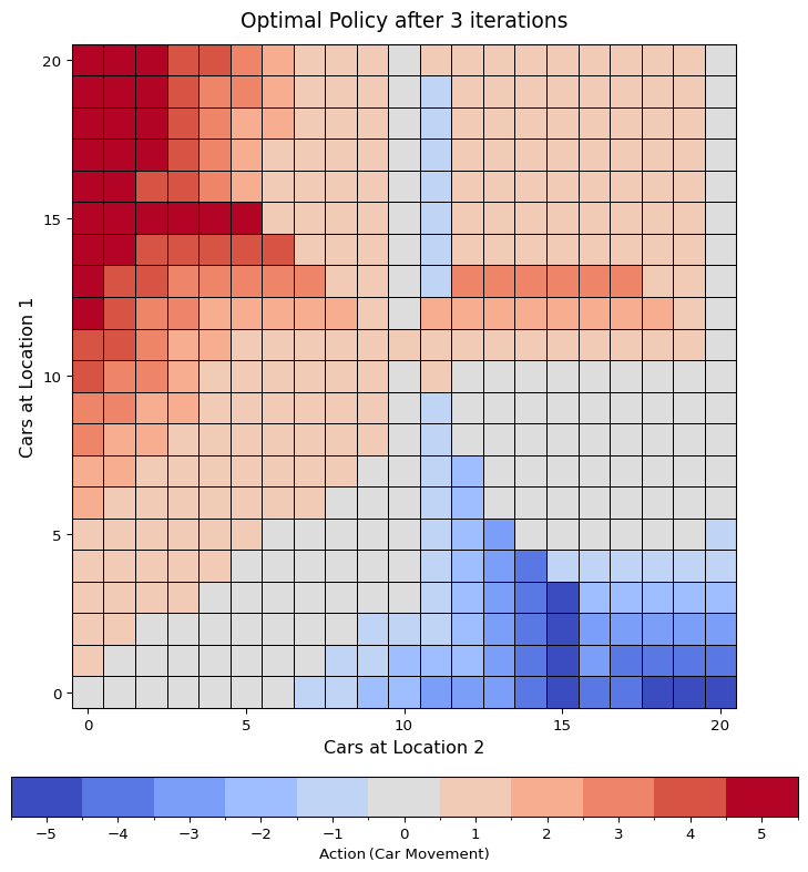
Example 4.2 Here we explore Example 4.2 from Sutton and Barto (2018) - Jack’s car rental.
Here’s a quick summary:
- two locations, each with a maximum of 20 cars (more cars added to a location magically vanish into thin air)
- during the day, a random amount of customers rent cars and then another random amount of customers return cars
- at the end of a day, up to 5 cars can be moved between the locations
- each car rented rewards 10
- each move car costs 2
- rentals and returns are Poisson distributed:
\(\lambda_{1,\text{rent}} =3\), \(\lambda_{1,\text{return}} =3\), \(\lambda_{2,\text{rent}} =4\), \(\lambda_{2,\text{return}} =2\)
We solve Jack’s car rental using policy iteration. The core computation in policy iteration is getting a state-action value from the state values, the one-step lookahead, which is used both in policy evaluation and policy improvement. This is the main performance bottleneck: \[ Q(s,a) = \sum_{s',r} p(s',r|s,a) [ r + \gamma V(s')] \]
This expression is good for theorizing about the algorithm but its direct implementation feels awkward and inefficient. In practice, it’s better to split the four-argument \(p(s',r|s,a)\) into expected immediate reward \(r(s,a)\) and the transition probability \(p(s'|s,a)\).
\[ \begin{split} Q(s,a) &= \sum_{s',r}p(s',r|s,a)r + \gamma\sum_{s',r}p(s',r|s,a)V(s') \\ &= r(s,a) + \gamma \sum_{s'}p(s'|s, a) V(s') \end{split} \]
Furthermore, we can make the algorithm more natural for this problem by introducing afterstates (Sutton and Barto 2018, sec. 6.8). Although we don’t use them to their full potential (we don’t learn an afterstate value function).
An afterstate is the environment state immediately after the agent’s action, but before the environment’s stochastic dynamics. This formulation is particularly effective when actions have deterministic effects. In Jack’s car rental, moving cars deterministically leads to an afterstate \(s \oplus a\), while the stochastic dynamics - rentals and returns - then determine the next state \(s'\).
The one-step lookahead using afterstates becomes: \[ Q(s,a) = c(a) + r(s \oplus a) + \gamma \sum_{s'} p(s'|s\oplus a)V(s'), \tag{4.4}\]
where \(c(a)\) is the cost of the, \(r(s \oplus a)\) is the expected immediate reward for the afterstate.
The following code is a nearly verbatim implementation of the policy iteration pseudocode, using Equation 4.4 for evaluation. (Select annotations to see inline explanations.)
# === policy iteration for Jack's car rental ===
from collections import namedtuple
from typing import Dict, List
from scripts.jacks_car_rental.jacks_car_rental import (
JacksCarRental,
State,
Action,
)
Policy = Dict[State, Action]
ValueFn = Dict[State, float]
def compute_state_action_value(
env: JacksCarRental, state: State, action: Action, value: ValueFn, γ: float
) -> float:
"""
Compute the expected one‐step return
"""
after_state, cost = env.move(state, action)
future_return = 0.0
for state_new in env.state_space:
p = env.get_transition_probability(after_state, state_new)
future_return += p * value[state_new]
return cost + env.get_expected_revenue(after_state) + γ * future_return
def policy_evaluation(
env: JacksCarRental, π: Policy, value: ValueFn, θ: float, γ: float
):
"""
Approximates the ValueFn from a deterministic policy
"""
while True:
Δ = 0.0
for s in env.state_space:
v_old = value[s]
v_new = compute_state_action_value(env, s, π[s], value, γ)
value[s] = v_new
Δ = max(Δ, abs(v_old - v_new))
if Δ < θ:
break
def policy_improvement(
env: JacksCarRental, π: Policy, value: ValueFn, γ: float
) -> bool:
"""
Improve a policy according to the provided value‐function
If no state's action changes, return True (policy is stable). Otherwise return False.
"""
stable = True
for s in env.state_space:
old_action = π[s]
best_action = max(
env.action_space,
key=lambda a: compute_state_action_value(env, s, a, value, γ),
)
π[s] = best_action
if best_action != old_action:
stable = False
return stable
PolicyIterationStep = namedtuple("PolicyIterationStep", ["policy", "values"])
def policy_iteration(env, θ, γ) -> List[PolicyIterationStep]:
optimal = False
history = []
# init policy and value-function
π: Policy = {s: 0 for s in env.state_space}
value: ValueFn = {s: 0.0 for s in env.state_space}
while not optimal:
# evaluation and save
policy_evaluation(env, π, value, θ, γ)
history.append(PolicyIterationStep(π.copy(), value.copy()))
# find better policy
optimal = policy_improvement(env, π, value, γ)
return history- 1
- Import the environment class and type aliases (State, Action) from the Jack’s car‐rental module.
- 2
- Since we are dealing with deterministic policies we can define Policy as a mapping.
- 3
- Implements the one‐step lookahead with afterstates (see Equation 4.4).
- 4
- Choose the action \(a\in \mathcal{A}(s)\) that maximises the one‐step lookahead; this is a concise way to do “\(\mathrm{argmax}_a \dots\)”” in Python
- 5
- The only slight change to the pseudocode: instead of just returning the optimal policy and its state-value function we return the history of policies.
Here is some more code just to be able to visualize our solution for Jack’s car rental problem…
Code
import numpy as np
import matplotlib.pyplot as plt
from matplotlib.colors import BoundaryNorm
from matplotlib import cm

from scripts.jacks_car_rental.jacks_car_rental import (
    JacksCarRentalConfig,
)


def plot_policy(title: str, config: JacksCarRentalConfig, π: dict):
    max_cars = config.max_cars
    max_move = config.max_move

    # Build a (max_cars+1)×(max_cars+1) integer grid of “action” values
    policy_grid = np.zeros((max_cars + 1, max_cars + 1), dtype=int)
    for (cars1, cars2), action in π.items():
        policy_grid[cars1, cars2] = action

    # X/Y coordinates for pcolormesh:
    x = np.arange(max_cars + 1)
    y = np.arange(max_cars + 1)
    X, Y = np.meshgrid(x, y)

    fig, ax = plt.subplots(figsize=(9, 9))

    # Discrete actions range
    actions = np.arange(-max_move, max_move + 1)
    n_colors = len(actions)

    # Create a “coolwarm” colormap with exactly n_colors bins
    cmap = plt.get_cmap("coolwarm", n_colors)

    # For a discrete colormap, we want boundaries at x.5, so that integer values
    # get mapped to their own color. Example: if max_move=2, actions = [-2, -1, 0, 1, 2],
    # then boundaries = [-2.5, -1.5, -0.5, 0.5, 1.5, 2.5].
    bounds = np.arange(-max_move - 0.5, max_move + 0.5 + 1e-6, 1)
    norm = BoundaryNorm(boundaries=bounds, ncolors=cmap.N)

    cax = ax.pcolormesh(
        X,
        Y,
        policy_grid,
        cmap=cmap,
        norm=norm,
        edgecolors="black",
        linewidth=0.4,
    )

    # Axis labels and title
    ax.set_xlabel("Cars at Location 2", fontsize=12)
    ax.set_ylabel("Cars at Location 1", fontsize=12)
    ax.set_title(title, fontsize=14, pad=12)

    # Square aspect ratio so each cell is a square:
    ax.set_aspect("equal")

    # Ticks every 5 cars
    step = 5
    ax.set_xticks(np.arange(0, max_cars + 1, step))
    ax.set_yticks(np.arange(0, max_cars + 1, step))

    # Colorbar (horizontal, at the bottom)
    cbar = fig.colorbar(
        cax,
        ax=ax,
        orientation="horizontal",
        pad=0.08,
        shrink=0.85,
        boundaries=bounds,
        ticks=actions,
        label="Action (Car Movement)",
    )
    cbar.ax.xaxis.set_label_position("bottom")
    cbar.ax.xaxis.tick_bottom()

    fig.tight_layout(rect=[0, 0.03, 1, 1])

    plt.show()


def plot_valueFn(title, config, val):
    """
    3D surface plot of the value function
    """
    max_cars = config.max_cars

    # Build a (max_cars+1)×(max_cars+1) grid of value estimates
    value_grid = np.zeros((max_cars + 1, max_cars + 1), dtype=float)
    for (l1, l2), v in val.items():
        value_grid[l1, l2] = v

    # Meshgrid for locations on each axis
    x = np.arange(max_cars + 1)
    y = np.arange(max_cars + 1)
    X, Y = np.meshgrid(x, y)

    fig = plt.figure(figsize=(11, 7))
    ax = fig.add_subplot(111, projection="3d")

    # Shaded surface plot
    surf = ax.plot_surface(
        X,
        Y,
        value_grid,
        rstride=1,
        cstride=1,
        cmap=cm.viridis,
        edgecolor="none",
        antialiased=True,
    )

    ax.set_xlabel("Cars at Location 2", fontsize=12, labelpad=10)
    ax.set_ylabel("Cars at Location 1", fontsize=12, labelpad=10)
    ax.set_title(title, fontsize=14, pad=12)
    ax.view_init(elev=35, azim=-60)

    fig.tight_layout()
    plt.show()
…and now we can solve it:
# === Solving Jack's car rental ===

# Hyperparameter for "training"
γ = 0.9
θ = 1e-5

# config and environment
config = JacksCarRentalConfig(max_cars=20)
env = JacksCarRental(config)

# do policy iteration
history = policy_iteration(env, θ, γ)

# print last (optimal) policy and its value function
plot_policy(
    f"Optimal Policy after {len(history)-1} iterations", config, history[-1].policy
)
plot_valueFn(f"Value function for optimal policy", config, history[-1].values)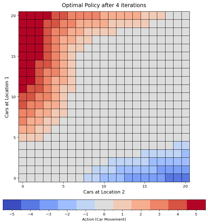
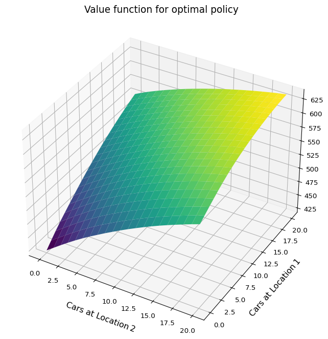
The runtime of this policy iteration is quite reasonable - just a few seconds. But considering we’re only dealing with \(441\) states, it highlights how dynamic programming is limited to small MDPs.
Another thought: although we now have the optimal solution, the meaning of the value function is still somewhat abstract. Mathematically it’s clear, but I couldn’t, for example, say whether Jack can pay his monthly rent with this business.
Exercise 4.4 The policy iteration algorithm Listing 4.2 has a subtle bug in that it may never terminate if the policy continually switches between two or more policies that are equally good. This is ok for pedagogy, but not for actual use. Modify the seudocode so that convergence is guaranteed.
Solution 4.4. If ties in the argmax are determined randomly, this could maybe result in a soft-lock when there are enough states with ties in their evaluation. Here we should add a condition that the policy is only changed if the change results in an actual improvement. Often in application there is an order on the actions, and we could also choose the smallest. However, this might also have consequences for the exploration of the algorithms.
So maybe the best solution is to only change the policy action if a better action improves the value by more than some \(\epsilon>0\):
Extra Paramater:
\(\epsilon\): small parameter determining of policy is stable
Policy Improvement
\(\text{policy-stable} \gets \mathrm{true}\)
for each \(s \in \mathcal{S}\):
\(\text{old-action} \gets \pi(s)\)
for each \(a \in \mathcal{A}(s)\):
\(Q(a) \gets \sum_{s',r} p(s',r | s,a) [ r + \gamma V(s') ]\)
\(\text{best-value} \gets \max_{a} Q(a)\)
if \(\text{best-value} - Q(\text{old-action}) > \epsilon\):
\(\pi(s) \gets a^*\) for which \(Q(a_*) = \text{best-value}\)
\(\text{policy‐stable} \gets \mathrm{false}\)
if policy‐stable:
return \(V \approx v_*\) and \(π ≈ π_*\)
else:
go to Policy Evaluation
Exercise 4.5 How would policy iteration be defined for action values? Give a complete algorithm for computing \(q_*\), analogous to Listing 4.2 for computing \(v_*\). Please pay special attention to this exercise, because the ideas involved will be used throughout the rest of the book.
Solution 4.5. The code depends on the convention that episodic tasks have an absorbing state that transitions only to itself and that generates only rewards of zero (Sutton and Barto 2018, sec. 3.4).
Parameter:
\(\theta\): a small positive number determining the accuracy of estimation
Initialisation:
\(Q(s,a) \in \mathbb{R}\), \(\pi(s) \in \mathcal{A}(s)\) arbitrarily, but \(Q(\mathrm{terminal},a) = 0\)
Policy Evaluation
Loop:
\(\Delta \gets 0\)
Loop for each \(s \in \mathcal{S}\) and \(a \in \mathcal{A}(s)\):
\(q \gets Q(s,a)\)
\(Q(s,a) \gets \sum_{s',r}p(s',r|s,a)[r + \gamma Q(s',\pi(s'))]\)
\(\Delta \gets \max(\Delta, |q - Q(s,a)|)\)
until \(\Delta < \theta\)
Policy Improvement
\(\text{policy-stable} \gets \mathrm{true}\)
For each \(s \in \mathcal{S}\):
\(\text{old-action} \gets \pi(s)\)
\(\pi(s) \gets \underset{a}{\mathrm{argmax}} \; Q(s,a)\)
If \(\text{old-action} \neq \pi(s)\), then \(\text{policy-stable} \gets \text{false}\)
If \(\text{policy-stable}\):
return \(Q \approx q_*\) and \(\pi \approx \pi_*\)
else:
go to Policy Evaluation
Exercise 4.6 Suppose you are restricted to considering only policies that are \(\varepsilon\)-soft, meaning that the probability of selecting each action in each state, \(s\), is at least \(\varepsilon/|\mathcal{A}(s)|\). Describe qualitatively the changes that would be required in each of the steps 3, 2, and 1, in that order, of the policy iteration algorithm Listing 4.2 for \(v_*\).
Solution 4.6. First of all, we are now dealing with a policy \(\pi(a|s)\) that assigns probabilities to actions instead of \(\pi(s)\) that choses an action.
For step 3, policy improvement, we assign to every possible action \(a\) a propability \(\varepsilon\), then the remainining propability \(1 - \varepsilon|\mathbfcal{A}(s)|\) to the actions that maximize the expression under the argmax.
For step 2, policy evaluation, we have to change the assignment to \(V(s) \gets \sum_{a} \pi(a|s) \sum_{s',r} p(s',r|s,a) [r + \gamma V(s')]\)
For step 1, initialisation, we have to make sure that each action gets a probability of at least \(\varepsilon\).
Exercise 4.7 Write a program for policy iteration and re-solve Jack’s car rental problem with the following changes. One of Jack’s employees at the first location rides a bus home each night and lives near the second location. She is happy to shuttle one car to the second location for free. Each additional car still costs $2, as do all cars moved in the other direction. In addition, Jack has limited parking space at each location. If more than 10 cars are kept overnight at a location (after any moving of cars), then an additional cost of $4 must be incurred to use a second parking lot (independent of how many cars are kept there). These sorts of nonlinearities and arbitrary dynamics often occur in real problems and cannot easily be handled by optimization methods other than dynamic programming. To check your program, first replicate the results given for the original problem.
Solution 4.7. We have already set up everyting in Example 4.2. I made sure in the implementation for the environment to include parameters for these changes.
# === solving Jack's car rental again ===
# Hyperparameter for "training"
γ = 0.9
θ = 1e-5

# config and environment
config = JacksCarRentalConfig(
    max_cars=20, free_moves_from_1_to_2=1, max_free_parking=10, extra_parking_cost=4
)
env = JacksCarRental(config)

# do policy iteration
history = policy_iteration(env, θ, γ)

# print last optimal policy
plot_policy(
    f"Optimal Policy after {len(history)-1} iterations", config, history[-1].policy
)
Interestingly this somewhat more complex problem, does need 1 less iteration than the original.
4.4 Value Iteration
Value iteration is policy iteration with a single sweep of policy evaluation per iteration.
In policy iteration, policy improvement is given by: \[ \pi_k(s) = \mathrm{argmax}_{a} \sum_{s',r} p(s',r|s,a)[r + \gamma v_k(s')] \]
This picks an action \(\hat{a}\) that gives the best one-step lookahead from the current value function.
Then, policy evaluation, uses the one-step lookahead for the updates: \[ v_{k+1}(s) = \sum_{s',r}p(s',r|s,\pi_k(s)) [r + \gamma v_k(s')] \]
But if we’re only doing one sweep, we may as well just plug in \(\hat{a}\) directly from the lookahead, which gives the maximum of this expression: \[ v_{k+1}(s) = \max_a \sum_{s',} p(s',r|s,a)[r + \gamma v_k(s')] \tag{4.5}\]
So, value iteration performs both greedy action selection and value backup in one go.
And here is the respective pseudocode:
Parameter:
\(\theta\): a small positive number determining the accuracy of estimation
Initialisation:
\(V(s)\) arbitrarily for \(s \in \mathcal{S}\), when episodic \(V(\mathrm{terminal}) = 0\)
Value Iteration
Loop:
\(\Delta \gets 0\)
Loop for each \(s \in \mathcal{S}\):
\(v \gets V(s)\)
\(V(s) \gets \max_a \sum_{s',r} p(s',p|s,a) [r + \gamma V(s')]\)
\(\Delta \gets \max(\Delta, |v - V(s)|)\)
until \(\Delta < \theta\)
Greedy Policy Extraction
Output a deterministic policy \(\pi \approx \pi_*\), such that
\(\pi(s) = \mathrm{argmax}_a \sum_{s',r} p(s',p|s,a) [r + \gamma V(s')]\)
4.4.1 gambler’s problem
Let’s talk about Example 4.3 from Sutton and Barto (2018) - the Gambler’s Problem. It gets its own little subsection because there’s actually quite a bit to say about it.
First, a quick summary of the MPD:
- the idea is to win a target amount \(N\) of chips by betting on coin flips
- non-terminal states are the current amount of chips (captial): \(\mathcal{S} = \{0,1,\dots,N\}\), and the terminal states are \(0\) and \(N\).
- actions are how mamny chips you wager (the stake): \(\mathcal{A}(s) = \{1,\dots, \min(s, N-s)\}\) for \(s \in \mathcal{S}\)
- the environment dynamics are \[ p(s' \mid a,s) = \begin{cases}p_{\mathrm{win}} &\text{if }s' = s+a\\1-p_{\mathrm{win}} &\text{if }s' = s-a \end{cases} \]
- rewards are 0 except for reaching the goal state \(N\), which gives a rewards of +1
- the task is episodic and undiscounted (\(\gamma = 1\))
The reward structure is set up so that the state-value function gives the probability of eventually reaching the goal from a given state: \[ v_\pi(s) = \mathbb{E}_\pi[G_t \mid S_t = s] = 1 \cdot \mathrm{Pr}_{\pi}(S_T = N \mid S_t = s) \]
So under any policy \(\pi\), the value of a state is just the probability of hitting \(N\) before hitting \(0\).
4.4.1.1 general remarks
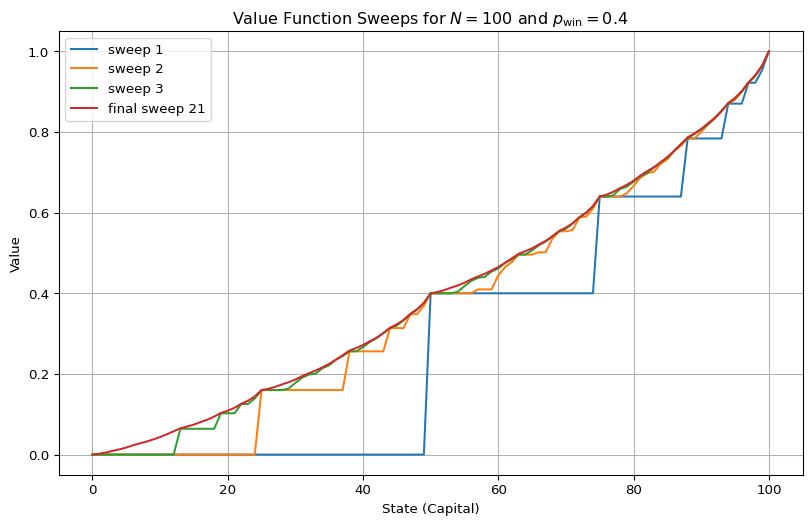
There’s a lot of content about this problem floating around online. Maybe that’s because it appears quite early in the book, or because it’s so simple to implement. Or maybe it’s because the problem hides a few trip wires. For one thing, if you implement it yourself without really understanding what’s going on, your correct solution might look completely wrong (see Figure 4.2 (b)).
A lot of the articles I’ve come across either lack substance or seem a bit confused - which is totally fair, but I personally prefer reading something more insightful when digging into a problem.
So here, I’m trying to give this a bit of extra depth.
4.4.1.2 no 0 stakes
Another issue you might stumble across is that the original example allows wagers of size 0. Which seems innocuous, but it actually complicates things when thinking about deterministic policies.
Since the problem is undiscounted, we have: \[ q_*(s,0) = v_*(s) = \max_a q_*(s,a) \]
So technically, wagering nothing could be considered an optimal action. However, any deterministic policy following such an action will not complete an episode.
Furthermore, zero stakes can also mess with value iteration. If we initialise the non-terminal states with a value greater than their optimal value, the algorithm will not update them, because it will just set \(v(s) = q(s,0)\).
It mostly leads to problems, so let’s leave them just out here.
4.4.1.3 one-step lookahead and environment
We’ll follow the design proposed by Sutton and Barto (2018): no rewards, and two terminal states:
- ruin: 0 capital, with value \(0\)
- win: 100 captial, with value \(1\)
The terminal states are not updated during value iteration, of course.
Given that, the one-step lookahead for stake \(s\) and wager \(a\) is especially simple to compute: \[ Q(s,a) = p_\mathrm{win} \cdot V(s+a) + (1-p_\mathrm{win}) \cdot V(s-a). \]
In code, it’s the environment’s responsibility to calculate the one-step lookaheads for a given state-value function (one_step_lookaheads), as well as to initialise the value function (make_initial_values). This gives us some nice encapsulation.
from typing import List

ValueFn = List[float]
State = int


class EnvGamblersProblem:
    def __init__(self, p_win: float, goal: int):
        self.p = p_win
        self.goal = goal
        self.non_terminal_states = list(range(1, goal))

    def make_initial_values(self, non_terminal_value: float) -> ValueFn:
        v = [0.0]  # terminal: ruin
        v.extend([non_terminal_value] * (self.goal - 1))  # non-terminals
        v.append(1.0)  # terminal: win
        return v

    def one_step_lookaheads(self, s: State, v: ValueFn):
        """returns a list of the q-values for state s.
        q[i] contains the value of betting an amount of i+1"""
        p = self.p
        goal = self.goal
        return [
            p * v[s + a] + (1 - p) * v[s - a] for a in range(1, min(s, goal - s) + 1)
        ]
4.4.1.4 solving the problem
Now we can implement value iteration, as described in Listing 4.5. We split the process into the two parts: value iteration and policy extraction.
I’ve modified the value iteration function so that it returns all intermediate value functions - the final one is the optimal state-value function.
def value_iteration_gamblers_problem(
env: EnvGamblersProblem, θ: float, init_value=0.0
) -> List[ValueFn]:
# **Init**
v = env.make_initial_values(init_value)
# **Value iteration**
value_functions = []
while True:
value_functions.append(v.copy())
Δ = 0.0
for s in env.non_terminal_states:
v_old = v[s]
v_new = max(env.one_step_lookaheads(s, v))
v[s] = v_new
Δ = max(Δ, abs(v_old - v_new))
if Δ < θ:
break
return value_functions
def get_greedy_policy(v: ValueFn, env: EnvGamblersProblem):
# ** Greedy Policy Extraction **
policy = {}
for s in env.non_terminal_states:
action_values = env.one_step_lookaheads(s, v)
greedy_action_idx = action_values.index(max(action_values))
policy[s] = greedy_action_idx + 1 # convert idx -> stake
return policy- 1
- this isn’t the most efficient way to compute the argmax of a list, but it’s fine for a simple problem like this.
Now, using the code below, we can solve the gambler’s problem for \(N = 100\) and \(p_\mathrm{win} = 0.4\).
# set up environment
env = EnvGamblersProblem(p_win=0.4, goal=100)

# run value_iteration
value_functions = value_iteration_gamblers_problem(env, 1e-12)

# optain optimal value function (result of last sweep)
v_star = value_functions[-1]

# optain optimal policy (greedy w.r.t to v_star)
policy_star = get_greedy_policy(v_star, env)
We plot the value function sweeps and a (somewhat strangely shaped) optimal policy below in Figure 4.2.
We’re not going to go into the mathematical analysis of the exact solution here, but if you’re curious about exact formulas for the value function, check out the section about ‘Bold Strategy’ for the game ‘Red and Black’ - which is apparently the mathematicans way of calling the gambler’s problem - in Siegrist (2023). 1
Code
import matplotlib.pyplot as plt
from typing import List, Tuple


def plot_value_function(
    value_functions: List[Tuple[str, ValueFn]],
    title: str = "Value Function Sweeps",
):
    plt.figure(figsize=(10, 6))

    for label, value_function in value_functions:
        plt.plot(range(0, len(value_function)), value_function, label=label)

    plt.xlabel("State (Capital)")
    plt.ylabel("Value")
    plt.title(title)
    plt.legend()
    plt.grid(True)
    plt.show()


# sweeps to plot
sweeps = (1, 2, 3, len(value_functions) - 1)
value_functions_with_labels = [
    (
        f"{"final " if i == len(value_functions) -1 else "" }sweep {i}",
        value_functions[i],
    )
    for i in sweeps
]
plot_value_function(
    value_functions_with_labels,
    title=r"Value Function Sweeps for $N=100$ and $p_\mathrm{win}=0.4$",
)
Code
import matplotlib.pyplot as plt
from typing import List, Tuple, Dict


def plot_policy(policy: Dict[int, int], title: str = "Policy"):
    plt.figure(figsize=(10, 6))

    states = sorted(policy.keys())
    actions = [policy[s] for s in states]
    plt.scatter(states, actions)

    plt.xlabel("State (Capital)")
    plt.ylabel("Action")
    plt.title(title)
    plt.grid(True)
    plt.show()


plot_policy(policy_star, title=r"An optimal policy for $N=100$ and p_\mathrm{win$ = 0.4$")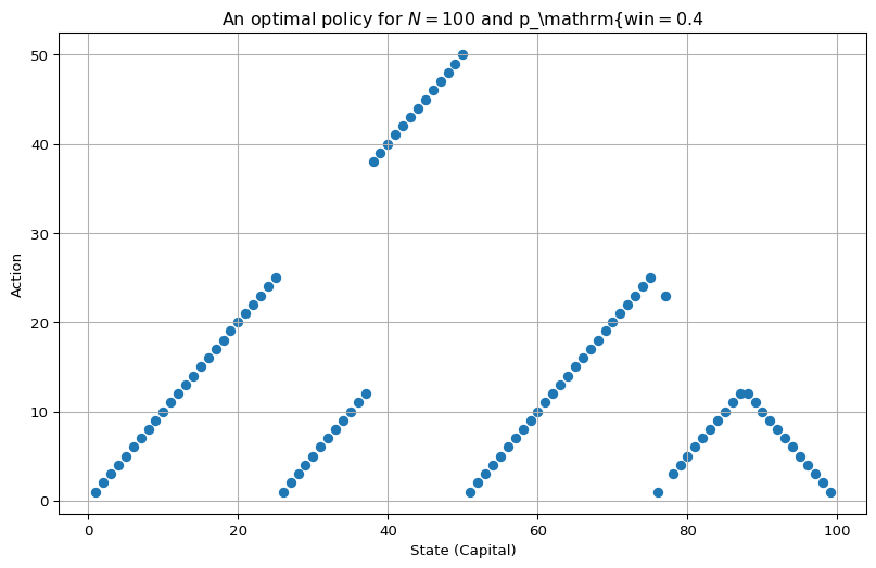
4.4.1.5 optimal actions
So, Figure 4.2 (b) looks jagged because, in some states, there are multiple optimal actions. The choice of which one is used isn’t governed by any particular logic in the implementation - it’s effectively decided by floating-point imprecision.
Here we want to answer this somewhat understated question from Sutton and Barto (2018, 84):
This policy [shown in Figure 4.3] is optimal, but not unique. In fact, there is a whole family of optimal policies, all corresponding to ties for the argmax action selection with respect to the optimal value function. Can you guess what the entire family looks like?
The short answer is: no, I can’t. It’s not something that’s easy to guess, in my view.
However, Siegrist (2023) gives an account of some well-developed theory addressing this question in. The section about bold play in the game Red and Black proves the existence of optimal strategies.
One such optimal strategy pattern applicable for all \(p_\mathrm{win} < 0.5\) and \(N\) is bold play, where you always bet the maximum amount possible: \[ B(s) := \max \mathcal{A}(s) = \min(\{s, N-s\}) \]
Actually, for any \(p_\mathrm{win} < 0.5\), all optimal actions are the same - only the underlying value functions change. The shape of \(B(s)\) is triangular, and if \(N\) is odd, it is the unique optimal policy, as seen in Figure 4.3 (c).
If \(N\) is even, then there exists a second-order bold strategy \(B_2\), which effectively applies divide and conquer to the problem (although I don’t have a really good intuition why it works). Create two subproblems, one from \(0\) to \(N/2\), and another from \(N/2\) to \(N\), each treated with their own bold strategy. It looks a bit like this (where \(\left\lfloor \frac{N}{4} \right\rfloor\) means \(N/4\) rounded down):
Code
import matplotlib.pyplot as plt
import numpy as np

# Define the x values
x = np.linspace(0, 1, 1000)


# Define the B_2(x)
def B2(x):
    return np.where(
        x < 0.25, x, np.where(x < 0.5, 0.5 - x, np.where(x < 0.75, -0.5 + x, 1 - x))
    )


# Create the plot
fig, ax = plt.subplots(figsize=(6, 4))
ax.plot(x, B2(x), color="blue")

# Highlight key points
ax.plot([0.5], [0.5], "o", color="blue")
ax.plot(
    [0.5], [0], "o", mfc="white", mec="blue", zorder=5, clip_on=False
)  # Draw over axis

# Add dashed grid lines for key points
ax.axhline(0.25, color="gray", linestyle="--", linewidth=0.5)
ax.axhline(0.5, color="gray", linestyle="--", linewidth=0.5)
ax.axvline(0.5, color="gray", linestyle="--", linewidth=0.5)
ax.plot([0.25, 0.5], [0.25, 0.5], "gray", linestyle="--", linewidth=0.5)
ax.plot([0.75, 0.5], [0.25, 0.5], "gray", linestyle="--", linewidth=0.5)

# Add axis labels and ticks
ax.set_xticks([0, 0.5, 1])
ax.set_xticklabels(["0", r"$\frac{N}{2}$", r"$N$"])
ax.set_yticks([0.25, 0.5])
ax.set_yticklabels([r"$\left\lfloor \frac{N}{4} \right\rfloor$", r"$\frac{N}{2}$"])

ax.set_xlabel(r"$s$")
ax.set_ylabel(r"$B_2(s)$", rotation=0, labelpad=15)

# Style the plot
ax.spines["top"].set_visible(False)
ax.spines["right"].set_visible(False)
ax.spines["left"].set_position("zero")
ax.spines["bottom"].set_position("zero")
ax.set_xlim(0, 1)
ax.set_ylim(0, 0.55)

plt.grid(False)
plt.tight_layout()
plt.show()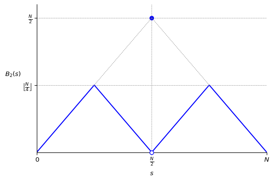
If \(N\) is divisible by \(4\), we can dividive and conquer again to get \(B_3\). This is exactly what we see in the original problem for \(N = 100\) (see Figure 4.3 (a)).
Basically, if \(N\) is divisible by \(2^\ell\) then \(B_\ell\) is an optimal stategy. In the limit, this family gives rise to a kind of fractal pattern of stacked diamonds (see Figure 4.3 (b)) - although these diamonds are missing their bottom tips, which would correspond to wagering 0.
So my finally answer to the inital question is. The family of optimal policies consists of any selection of actions from the bold-strategy hierarchy: \(B\) (one big triangle), \(B_2\) (two triangles), and \(B_3\) (four triangles).
Code
from dataclasses import dataclass
from typing import Dict, List


def get_greedy_actions(v, env, ε):
    optimal_actions = {}
    for s in env.non_terminal_states:
        q_values = env.one_step_lookaheads(s, v)
        max_value = max(q_values)
        bests = []
        for a, q in enumerate(q_values):
            if max_value - q < ε:
                bests.append(a + 1)
        optimal_actions[s] = bests

    return optimal_actions


@dataclass
class MultiPolicy:
    actions: Dict[int, List[int]]  # state -> list of stakes
    name: str = None
    marker: str = "o"
    size: int = None


def plot_multi_policy(multi_policies: List[MultiPolicy], title: str):
    plt.figure(figsize=(10, 6))

    draw_legend = False

    for pol in multi_policies:
        pts = [(s, a) for s, al in pol.actions.items() for a in al]
        states, acts = zip(*pts)
        if pol.name:
            draw_legend = True
        plt.scatter(
            states,
            acts,
            marker=pol.marker,
            s=pol.size,
            label=pol.name,
        )

    plt.xlabel("State (Capital)")
    plt.ylabel("Action (Stake)")
    if draw_legend:
        plt.legend()
    plt.title(title)
    plt.grid(True)
    plt.show()


best_actions = get_greedy_actions(v_star, env, 1e-8)

best_minimal_actions = {}
for s in best_actions:
    best_min = min(best_actions[s])
    best_minimal_actions[s] = [best_min]

optimals = [
    MultiPolicy(best_actions, name="optimal actions"),
    MultiPolicy(best_minimal_actions, name="third-order bold strategy", marker="x", size=30),
]
plot_multi_policy(optimals, title="Optimal Actions for N=100")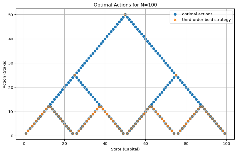
Code
goal = 5 * 32
env = EnvGamblersProblem(p_win=0.4, goal=goal)
value_functions = value_iteration_gamblers_problem(env, 1e-14)
v_star = value_functions[-1]
best_actions = get_greedy_actions(v_star, env, 1e-8)
plot_multi_policy([MultiPolicy(best_actions, size=12)], title=f"Optimal actions for N={goal}")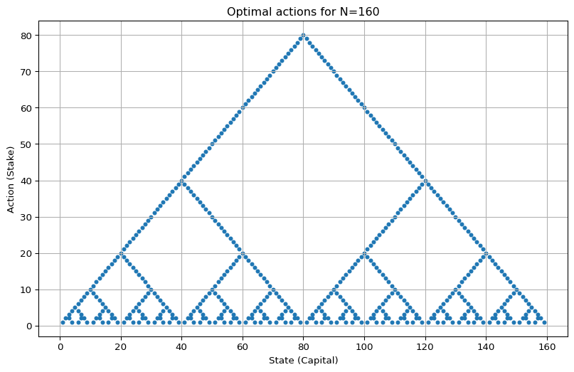
Code
goal = 101
env = EnvGamblersProblem(p_win=0.4, goal=goal)
value_functions = value_iteration_gamblers_problem(env, 1e-12)
v_star = value_functions[-1]
best_actions = get_greedy_actions(v_star, env, 1e-8)
plot_multi_policy([MultiPolicy(best_actions)], title=f"Optimal actions for N={goal}")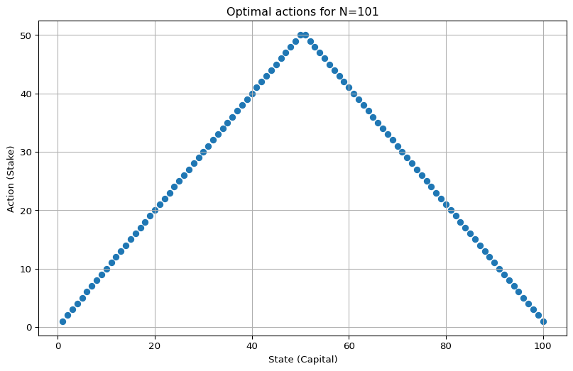
4.4.1.6 gambler’s ruin
Check out the value function in Figure 4.2 (a). It looks like, even though a single coin flip is stacked against the gambler with \(p_\mathrm{win} = 0.4\), if they start with a large capital, say 80 chips, they still reach the goal of \(N = 100\) about 70% of the time. Doesn’t sound too bad. But of course, if they succeed, they only win 20 chips. If they lose, they lose 80 chips.
One general result that captures this asymmetry is gambler’s ruin, which states essentially that when the odds are stacked against the gambler, there is no strategy to turn the odds in their favour.
We can make this concrete by calculating the expected monetary return when following the optimal strategy, starting with \(s\) chips: \[ \mathbb{E}_{\pi_*}[S_T - S_0 \mid S_0 = s] = p_{\mathrm{goal}}(N-s) + (1-p_{\mathrm{goal}})(-s), \]
where \[ p_{\mathrm{goal}}(s) = \mathrm{Pr}_{\pi_*}(S_T = N \mid S_0 = s) = v_*(s). \]
Let’s compute and plot it for \(p = 0.4\) and \(N = 100\):
Code
goal = 100
p_win = 0.4
env = EnvGamblersProblem(p_win=p_win, goal=goal)
value_functions = value_iteration_gamblers_problem(env, 1e-12)
v_star = value_functions[-1]
expected_profit = [
    value * (env.goal - s) - (1 - value) * s for s, value in enumerate(v_star)
]


plt.figure(figsize=(10, 6))

plt.plot(range(0, len(expected_profit)), expected_profit)
plt.xlabel("Startign Capital")
plt.ylabel("Expected profit")
plt.title(
    r"Profit when following an optimal strategy for $N = 100$ and $p_\mathrm{win} = 0.4$"
)
plt.grid(True)
plt.show()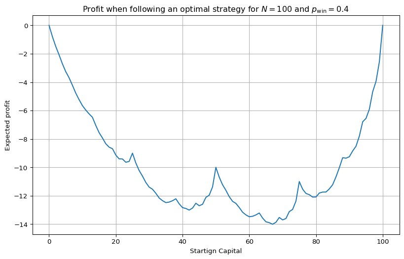
Even though the plot shows a nice (fractal-looking) w shape, you’re expected to lose chips, no matter what your initial capital is.
If you have to play, then the best is to start with either very low or very high capital - this is not financial advice though 🥸.
As a risk-averse person, my actual advice is: start with \(0\) or \(100\) chips - i.e., don’t play at all.
4.4.1.7 gambler’s fortune
When we stack the game in favour of the gambler \(p_{\mathrm{win}} > 0.5\) everything becomes somewhat easier.
There is just one optimal strategy, timid play, that is, always bet exactly one coin \[ \pi_*(s) = 1. \]
The value function in this case has a clean analytical form: \[ v(s) = \frac{1 - \left(\frac{1-p}{p}\right)^s}{1 - \left(\frac{1-p}{p}\right)^N} \]
And… well, that’s basically it. Winnig all the time doesn’t require any creative policies.
4.4.1.8 floating point imprecissions
There’s one interesting thing about the gambler’s fortune case. The high win probabilities can lead to floating point imprecisions.
When we run value iteration with \(N = 100\) and \(p_\mathrm{win} = 0.6\), these imprecisions can bleed into the computed optimal policy.
Code
env = EnvGamblersProblem(p_win=0.6, goal=100)
value_functions = value_iteration_gamblers_problem(env, 1e-12)
v_star = value_functions[-1]
plot_value_function([("optimal value function", v_star)])
best_actions = get_greedy_actions(v_star, env, 1e-10)
plot_multi_policy([MultiPolicy(best_actions)], title="bla")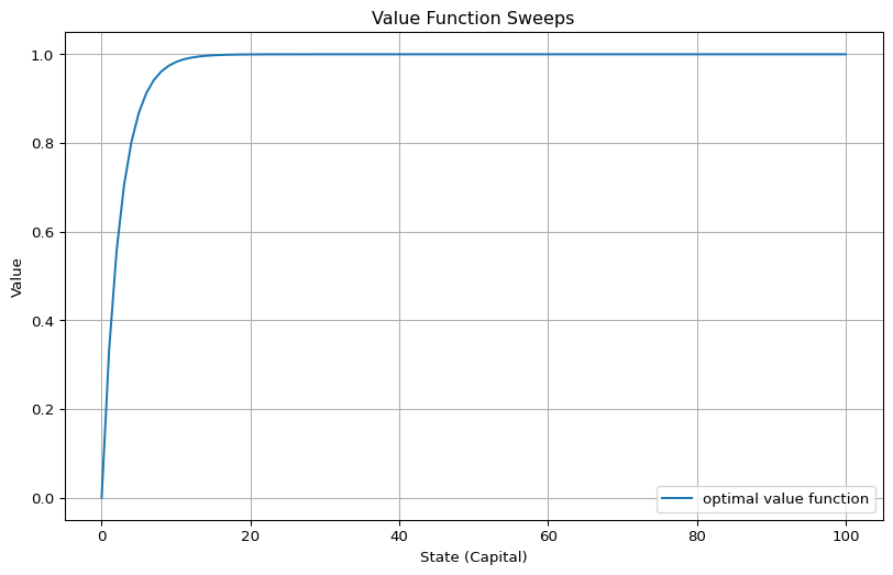
The value function approaches \(1\) very quickly. That means from a certain point onward, the \(q(s, a)\) values are all indistinguishably close to \(1\)…
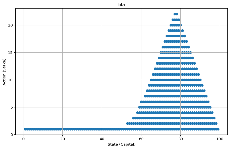
…which leads to floating point imprecisions during optimal action selection. The code ends up including some sub-optimal actions.
Two thoughts on this:
- Practically speaking, this isn’t really a problem. When all candidate actions yield a value practically indistinguishable from the max, it doesn’t matter which one we take. They’re all effectively optimal.
- Theoretically, it’s a useful reminder: a computation is not a proof. It can return wrong answers. Our algorithms produce approximations of the optimal policy, and here it’s harmless, but we should keep it in mind.
This kind of issue always arises when the \(q\)-values are close together. You can also see it with very low win probabilities:
Code
env = EnvGamblersProblem(p_win=0.01, goal=128)
value_functions = value_iteration_gamblers_problem(env, 1e-12)
v_star = value_functions[-1]
best_actions = get_greedy_actions(v_star, env, 1e-8)
plot_multi_policy([MultiPolicy(best_actions)], title=r"$p_\mathrm{win} = 0.01$ and $N=100$")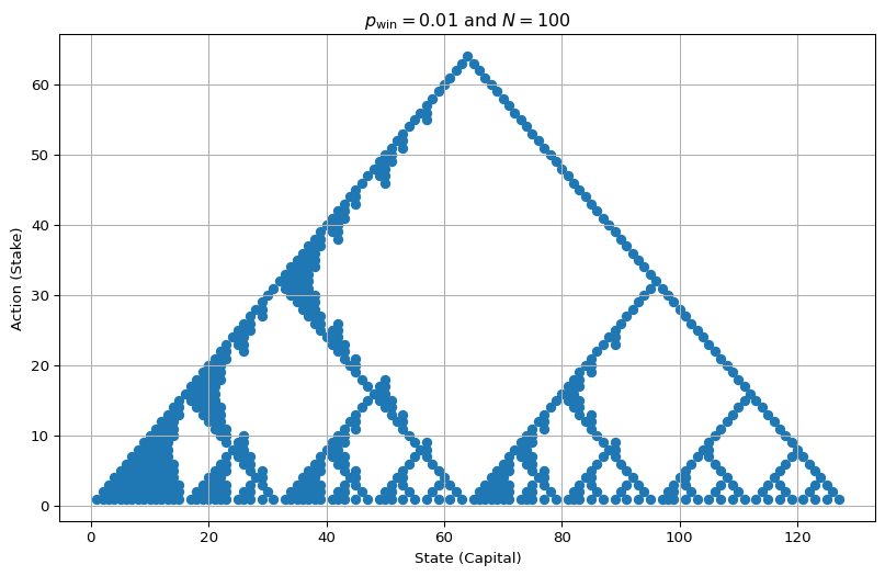
Note: For illustration, I’ve deliberately used ‘large’ \(\varepsilon\) values (\(10^{-10}\) for \(p_\mathrm{win} = 0.6\) and \(10^{-8}\) for \(p_\mathrm{win} = 0.01\)) when deciding which actions to treat as equally good, that is, if \(|q(s,a) - q(s,a')| < \varepsilon\), we consider both actions equally good.
Exercise 4.8 Why does the optimal policy for the gambler’s problem have such a curious form? In particular, for capital of 50 it bets it all on one flip, but for capital of 51 it does not. Why is this a good policy?
Solution 4.8. As discussed in Section 4.4.1.5, there is no single optimal policy.
For capital 50, there’s only one optimal action - bet it all. This reflects the general strategy of bold play, which intuitively limits the number of steps (and thus the compounding risk) needed to reach the goal.
For capital 51, though, there are two optimal actions: continue being bold (bet 49), or - as shown in the policy from Sutton and Barto (2018) - just bet 1.
That both are equally good and optimal follows from the maths. But in my opinion, any simple intuitive explanation is just a posteriori justification of the mathematical facts.
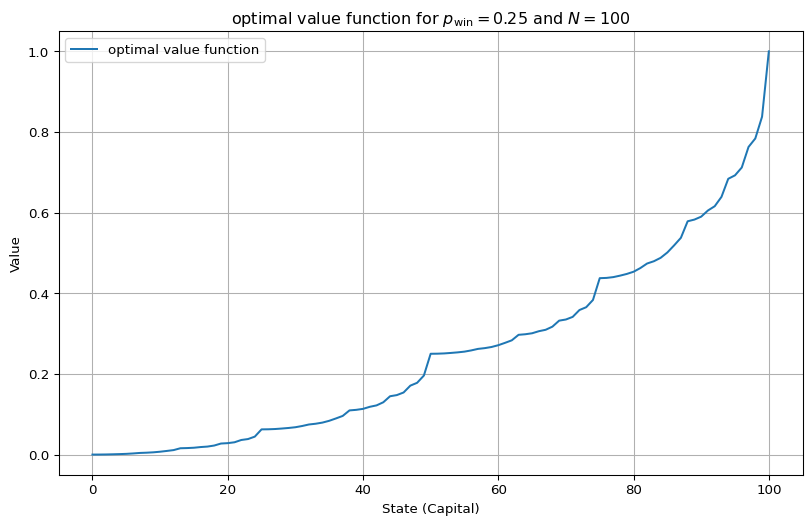
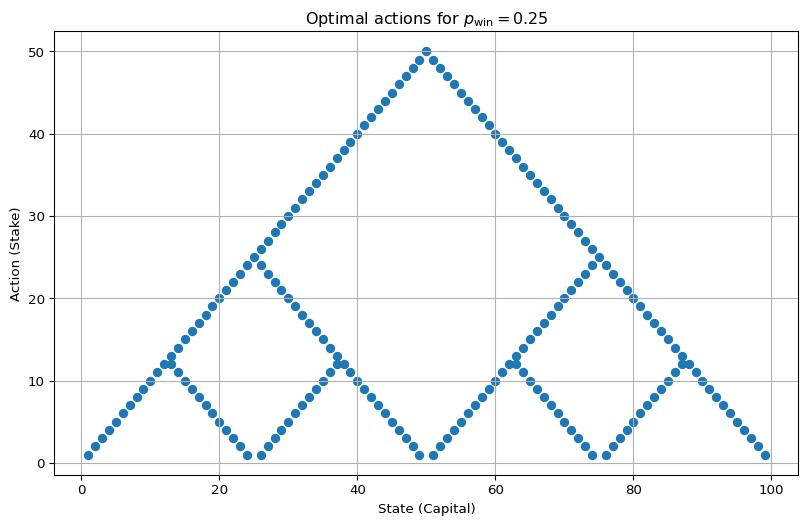
Exercise 4.9 Implement value iteration for the gambler’s problem and solve it for \(p_\mathrm{win} = 0.25\) and \(p_{\mathrm{win}} = 0.55\). In programming, you may find it convenient to introduce two dummy states corresponding to termination with capital of \(0\) and \(100\), giving them values of \(0\) and \(1\) respectively. Show your results graphically, as in Figure 4.2. Are your results stable as \(\theta \to 0\)?
Solution 4.9. Here are the computed solutions - both the state-value functions and the optimal policies. For the policies, we show all optimal actions.
There are no surprises here; everything behaves as previously discussed.
Code
env = EnvGamblersProblem(p_win=0.25, goal=100)
value_functions = value_iteration_gamblers_problem(env, 1e-12)
v_star = value_functions[-1]
best_actions = get_greedy_actions(v_star, env, 1e-10)
plot_value_function([("optimal value function", v_star)], title=r"optimal value function for $p_\mathrm{win} = 0.25$ and $N=100$")
plot_multi_policy(
[MultiPolicy(best_actions)], title=r"Optimal actions for $p_\mathrm{win} = 0.25$"
)
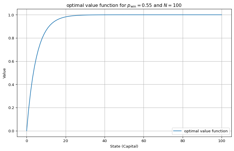
env = EnvGamblersProblem(p_win=0.55, goal=100)
value_functions = value_iteration_gamblers_problem(env, 1e-12)
v_star = value_functions[-1]
best_actions = get_greedy_actions(v_star, env, 1e-10)
plot_value_function([("optimal value function", v_star)], title=r"optimal value function for $p_\mathrm{win} = 0.55$ and $N=100$")
plot_multi_policy(
[MultiPolicy(best_actions)], title=r"$Optimal actions for p_\mathrm{win} = 0.55$"
)
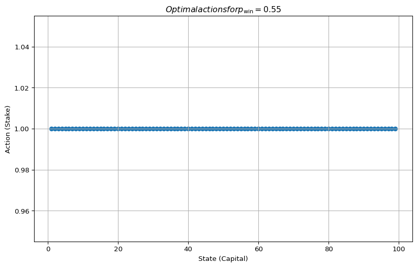
All used \(\theta = 10^{-10}\)
These solutions are not stable as \(\theta \to 0\) (pushing \(\theta < 10^{-18}\) seems to be numerically fragile).
If we go that low, we get residual differences in the values, which can make some optimal actions appear non-optimal:
Code
env = EnvGamblersProblem(p_win=0.25, goal=100)
value_functions = value_iteration_gamblers_problem(env, 1e-18)
v_star = value_functions[-1]
best_actions = get_greedy_actions(v_star, env, 1e-16)
plot_multi_policy(
    [MultiPolicy(best_actions)], title=r"$p_\mathrm{win} = 0.25$ and $N=100$ with $\theta = 10^{-18}"
)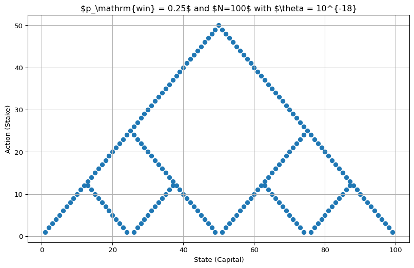
That said, unlike the issues in Section 4.4.1.8, this doesn’t lead to wrong policies - they still contain only optimal actions.
Exercise 4.10 What is the analog of the value iteration update Equation 4.5 for action values, \(q_{k+1}(s, a)\)?
From the greedy policy update: \[ \pi_k(s) = \mathrm{argmax}_a q_k(s,a) \] and the action-value Bellman update: \[ q_{k+1}(s,a) = \sum_{s',r}p(s',r|s,a) [r + \gamma Q(s', \pi_k(s'))] \] we get the action-value version of the value iteration update: \[ q_{k+1}(s, a) = \sum_{s',r} p(s',r|s,a)[r + \gamma \max_{a'} Q(s',a')] \]
4.5 Asynchronous Dynamic Programming
Nothing to add here,
4.6 Generalized Policy Iteration
nor here,
4.7 Efficiency of Dynamic Programming
or here,
4.8 Summary
and not even here.
Siegrist, Kyle. 2023. “Probability, Mathematical Statistics, Stochastic Processes.” https://www.randomservices.org/random/index.html.
Sutton, Richard S., and Andrew G. Barto. 2018. Reinforcement Learning: An Introduction. Second edition. Adaptive Computation and Machine Learning Series. Cambridge, MA: MIT Press. https://mitpress.mit.edu/9780262039246/reinforcement-learning/.
They use a continuous version of the gambler’s problem, but the continous value function \(F\) can be translated by \(v_\ast(s) = F(\frac{x}{N})\). That’s because the optimal strategy, ‘bold play’, can also be used in the discrete caes.↩︎