2  Multi-armed Bandits

(Some imports for python, can be ignored)

from dataclasses import dataclass, field
import numpy as np
import matplotlib.pyplot as plt
from typing import Sequence, Tuple

2.1 A k-armed Bandit Problem

The k-armed bandit problem is a very simple example that already introduces a key structure of reinforcement learning: the reward depends on the action taken. It’s technically not a full Markov chain (more on that in Section 3.1)—since there are no states or transitions—but we still get a sequence of dependent random variables \(A_1, R_1, A_2, \dots\), where each reward \(R_t\) depends on the corresponding action \(A_t\).

The true value of an action is defined as: \[ q_*(a) := \mathbb{E}[ R_t \mid A_t = a]. \]

The time index here doesn’t play a special role as the action-reward probabilities in the armed bandit are stationary. You can think of it as “when \(a\) is picked”—that is, the expected reward when action \(a\) is chosen.

If you’re feeling queasy about the conditional expected value, here’s a quick refresher on the relevant notation and concepts.

random variables and probability

The foundations of all processes we discuss here are discrete probability spaces \((\Omega, \mathrm{Pr})\). \(\Omega\) is the set of all possible trajectories—that is, complete sequences of outcomes for the random variables in a single run of the process—and \(\mathrm{Pr}\) assigns a probability to each trajectory. That is, \[ \mathrm{Pr}\colon \Omega \to [0,1] \quad \text{with} \quad \sum_{\omega \in \Omega} \mathrm{Pr}(\omega) = 1. \]

The random variables \(X\) are simply functions \(X\colon \Omega \to \mathcal{X}\) from \(\Omega\) to a result space \(\mathcal{X}\).

We follow the convention of Sutton and Barto (2018): random variables are written in capital letters, and their possible values are in lowercase.

If we want to refer to the concrete outcome of a single trajectory (which we actually don’t often do in theory crafting), we evaluate random variables on a specific \(\omega \in \Omega\), which fixes their values. So an arbitrary trajectory looks like this \(A_1(\omega), R_1(\omega), A_2(\omega), R_2(\omega) \dots\)

Let’s bring up two common conventions we can find in \(\mathbb{E}[ R_t \mid A_t = a]\):

1. We usually omit the argument \(\omega\) when referring to the value of a random variable. This is what makes the randomness implicit in a random variable \(X\). This mathematically conflates the function \(X ⁣\colon\Omega\to \mathcal{X}\) with the value \(X(\omega)\), but context sorts that out.
2. When writing functions of sets, we abbreviate expressions like \(F({\omega \in \Omega : \text{statement true in }\omega})\) to simply \(F(\text{statement})\).

With both conventions in play, we can see that \(\mathrm{Pr}(X = x)\) is just shorthand for \(\mathrm{Pr}(\omega \in \Omega : X(\omega) = x)\)

conditional probability

The reward \(R_t\)​ depends on the action \(A_t\)​ taken. If we know the value of \(A_t\), then the conditional probability that \(R_t=r\) given \(A_t = a\) is: \[ \mathrm{Pr}(R_t = r \mid A_t = a) = \frac{\mathrm{Pr}(R_t = r, A_t = a)}{\mathrm{Pr}(A_t = a)}, \]

where the comma denotes conjunction of the statements.

This is only well-defined if \(\mathrm{Pr}(A_t = a) > 0\) but that’s a technicality we won’t worry too much about—it won’t bite us.

expected value

Real-valued random variables like \(R_t\colon \Omega \to \mathbb{R}\) have an expected value—also called the mean—\(\mathbb{E}[R_t]\), defined as: \[ \mathbb{E}[ R_t ] := \sum_{\omega \in \Omega} R_t(\omega) \mathrm{Pr}(\omega) \]

A more commonly used form—sometimes called the “law of the unconscious statistician” (see appendix Theorem 2.1)—is: \[ \mathbb{E}[R_t] = \sum_{r \in \mathcal{R}} r \; \mathrm{Pr}(R_t = r), \]

To compute a conditional expectation, we just switch probabilities with conditional probabilities: \[ \mathbb{E}[R_t \mid A_t = a] = \sum_{\omega \in \Omega} R_t(\omega) \mathrm{Pr}(\omega \mid A_t = a). \]

Or, using the more practical LOTUS form: \[ \mathbb{E}[R_t \mid A_t = a] = \sum_{r \in \mathcal{R}} r \; \mathrm{Pr}(R_t = r \mid A_t = a). \]

To close the loop, a more explicit formulation of the true value of an action is: \[ q_*(a) = \sum_{r \in \mathcal{R}} r \; \frac{\mathrm{Pr}(R_t = r, A_t = a)}{\mathrm{Pr}(A_t = a)} \] (This form is arguably less intuitive, but it’s included here to jog our memory.)

2.2 Action-value Methods

This part always trips me up, so let me clarify it for myself: \(Q_t(a)\) is the estimated value of action \(a\) prior to time \(t\), so not included are \(A_t\) and it’s corresponding reward \(R_t\).

Instead, \(A_t\) is selected based on the current estimates \(\{Q_{t}(a):a \in \mathcal{A}\}\). For example, our algorithm could pick \(A_t\)​ greedily as \(A_t:=\mathrm{argmax}_{a \in \mathcal{A}} Q_t(a)\), or \(\varepsilon\)-greedily.

Exercise 2.1 In \(\varepsilon\)-greedy action selection, for the case of two actions and \(\varepsilon = 0.5\), what is the probability that the greedy action is selected?

Solution 2.1. The total probability of selecting the greedy action is: \[ \mathrm{Pr}(\text{greedy action}) + \mathrm{Pr}(\text{exploratory action}) \cdot \frac{1}{2} = 0.75 \]

2.3 The 10-armed Testbed

The 10-armed testbed will accompany us through the rest of this chapter (I had to keep it variable in size just for the sake of generalization though).

# === the armed bandit ===
class ArmedBandit:
    """k-armed Gaussian bandit."""
    def __init__(self, action_mu, action_sd, seed):
        self.action_mu = np.asarray(action_mu, dtype=np.float64)
        self.action_sd = np.asarray(action_sd, dtype=np.float64)
        self.seed = seed
        self.rng = np.random.default_rng(self.seed)

    def pull_arm(self, action):
        return self.rng.normal(loc=self.action_mu[action], scale=self.action_sd)

And here’s the code for the sample-average bandit algorithm. For clarity, I’ll refer to this and upcoming algorithms as ‘agents’, given their autonomous implementation. Note that we’re also using the incremental implementation from section 2.4.

# === the simple average bandit agent ===
class SampleAverageBanditAgent:
    def __init__(self, Q1, ε, seed=None):
        self.rng = np.random.default_rng(seed)
        self.num_actions = len(Q1) 
        self.Q1 = np.asarray(Q1, dtype=np.float64)  # initial action-value estimates
        self.ε = ε  
        self.reset()

    def reset(self):
        self.Q = self.Q1.copy()
        self.counts = np.zeros(self.num_actions, dtype=int)

    def act(self, bandit):
        # ε-greedy action selection
        if self.rng.random() < self.ε:
            action = self.rng.integers(self.num_actions)
        else:
            action = np.argmax(self.Q)

        # take action and observe the reward
        reward = bandit.pull_arm(action)

        # update count and value estimate
        self.counts[action] += 1
        α = 1 / self.counts[action]
        self.Q[action] += α * (reward - self.Q[action])

        return (action, reward)

Next, I’ll define an experiment function bandit_experiment that we’ll use throughout this chapter. In short, it takes multiple agents, length of each episode, and the number of episodes, then executes these agents repeatedly in a shared bandit environment, which gets reset after each episode. It returns two arrays: the average reward per step and the percentage of optimal actions taken per step—both averaged over all runs. These results can then be visualised using the plotting functions also provided. You don’t have to read the code unless you’re curious…

# === the core bandit experiment ===

# --- config
@dataclass
class Config:
    bandit_num_arms: int = 10
    bandit_setup_mu: float = 0.0
    bandit_setup_sd: float = 1.0
    bandit_action_sd: float = 1.0
    bandit_value_drift: bool = False
    bandit_value_drift_mu: float = 0.0
    bandit_value_drift_sd: float = 0.0
    exp_steps: int = 1_000
    exp_runs: int = 200
    exp_seed: int = 0


# -- core experiment
def bandit_experiment(agents, config: Config) -> Tuple[np.ndarray, np.ndarray]:
    """
    Run `exp_runs` × `exp_steps` episodes and return:

    average_rewards         shape = (len(agents), exp_steps)
    optimal_action_percent  shape = (len(agents), exp_steps)
    """
    rng = np.random.default_rng(config.exp_seed)
    num_agents = len(agents)
    average_rwds = np.zeros((num_agents, config.exp_steps))
    optimal_acts = np.zeros((num_agents, config.exp_steps))

    # allocate a single bandit and reuse its object shell
    bandit = ArmedBandit(
        action_mu=np.empty(config.bandit_num_arms),  # placeholder
        action_sd=config.bandit_action_sd,
        seed=config.exp_seed,
    )

    for run in range(config.exp_runs):
        # fresh true values for this run
        bandit.action_mu[:] = rng.normal(
            config.bandit_setup_mu, config.bandit_setup_sd, size=config.bandit_num_arms
        )
        best_action = np.argmax(bandit.action_mu)

        # reset all agents
        for agent in agents:
            agent.reset()

        # vectorised drift noise: shape = (exp_steps, bandit_num_arms)
        if config.bandit_value_drift:
            drift_noise = rng.normal(
                config.bandit_value_drift_mu,
                config.bandit_value_drift_sd,
                size=(config.exp_steps, config.bandit_num_arms),
            )

        # main loop
        for t in range(config.exp_steps):
            for i, agent in enumerate(agents):
                act, rwd = agent.act(bandit)
                average_rwds[i, t] += rwd
                optimal_acts[i, t] += act == best_action

            if config.bandit_value_drift:
                bandit.action_mu += drift_noise[t]
                best_action = np.argmax(bandit.action_mu)

    # mean over runs
    average_rwds /= config.exp_runs
    optimal_acts = 100 * optimal_acts / config.exp_runs
    return average_rwds, optimal_acts


# --- thin plotting helpers
def plot_average_reward(
    average_rewards: np.ndarray,
    *,
    labels: Sequence[str] | None = None,
    ax: plt.Axes | None = None,
) -> plt.Axes:
    """One line per agent: average reward versus step."""
    if ax is None:
        _, ax = plt.subplots(figsize=(8, 4))

    steps  = np.arange(1, average_rewards.shape[1] + 1)
    if labels is None:
        labels = [f"agent {i}" for i in range(average_rewards.shape[0])]

    for i, lbl in enumerate(labels):
        ax.plot(steps, average_rewards[i], label=lbl)

    ax.set_xlabel("Step")
    ax.set_ylabel("Average reward")
    ax.set_title("Average reward per step")
    ax.grid(alpha=0.3, linestyle=":")
    ax.legend()
    return ax


def plot_optimal_action_percent(
    optimal_action_percents: np.ndarray,
    *,
    labels: Sequence[str] | None = None,
    ax: plt.Axes | None = None,
) -> plt.Axes:
    """One line per agent: % optimal action versus step."""
    if ax is None:
        _, ax = plt.subplots(figsize=(8, 4))

    steps  = np.arange(1, optimal_action_percents.shape[1] + 1)
    if labels is None:
        labels = [f"agent {i}" for i in range(optimal_action_percents.shape[0])]

    for i, lbl in enumerate(labels):
        ax.plot(steps, optimal_action_percents[i], label=lbl)

    ax.set_xlabel("Step")
    ax.set_ylabel("% optimal action")
    ax.set_title("Optimal-action frequency")
    ax.grid(alpha=0.3, linestyle=":")
    ax.legend()
    return ax

…, but it’s still helpful to see such an experiment in action. We can, for example, recreate Figure 2.2 (Sutton and Barto 2018). It compares the performance of a greedy agent (\(\varepsilon = 0\)), and two \(\varepsilon\)-greedy agents with \(\varepsilon =0.1\) and \(\varepsilon=0.01\). We let them run for a couple of steps and then repeat this process for a couple of runs to get a smoother curve.

# === comparison greediness ===
# configuration of the experiment
config = Config(
    exp_steps=1_000,
    exp_runs=2_000)

# initialize agents with different epsilon values
epsilons = [0.0, 0.1, 0.01]
agents = [SampleAverageBanditAgent(Q1=np.zeros(config.bandit_num_arms), ε=ε, seed=config.exp_seed) for ε in epsilons]

# run bandit experiment
avg_rwd, opt_pct = bandit_experiment(
    agents,
    config    
)

# plots
labels = [f"ε={e}" for e in epsilons]

plot_average_reward(avg_rwd, labels=labels)
plt.tight_layout()
plt.show()

plot_optimal_action_percent(opt_pct, labels=labels)
plt.tight_layout()
plt.show()

(a) The average reward.

(b) The percentage of optimal step selection

Figure 2.1: This is like Figure 2.2 (Sutton and Barto 2018): the average performance of different ε-greedy sample average methods over 2000 runs. On the 10-armed testbed.

Out of curiosity, let’s see what happens when we have only one run (so it’s not the average anymore but just the reward). It’s a mess, wow. Without averaging over a couple of runs, we can’t make out anything.

# === experiment with only one run ===
config = Config(
    exp_steps=1_000,
    exp_runs=1)

epsilons = [0.0, 0.1, 0.01]
agents = [SampleAverageBanditAgent(Q1=np.zeros(config.bandit_num_arms), ε=ε, seed=config.exp_seed) for ε in epsilons]
avg_rwd, opt_pct = bandit_experiment(
    agents,
    config
)

plot_average_reward(avg_rwd, labels=[f"ε={e}" for e in epsilons])
plt.tight_layout()
plt.show()

Exercise 2.2 (Bandit example) Consider a k-armed bandit problem with k = 4 actions, denoted 1, 2, 3, and 4. Consider applying to this problem a bandit algorithm using \(\varepsilon\)-greedy action selection, sample-average action-value estimates, and initial estimates of \(Q_1(a) = 0\), for all a. Suppose the initial sequence of actions and rewards is \(A_1 = 1\), \(R_1 = -1\), \(A_2 = 2\), \(R_2 = 1\), \(A_3 = 2\), \(R_3 = -2\), \(A_4 = 2\), \(R_4 = 2\), \(A_5 = 3\), \(R_5 = 0\). On some of these time steps the \(\varepsilon\) case may have occurred, causing an action to be selected at random. On which time steps did this definitely occur? On which time steps could this possibly have occurred?

Solution 2.2. Step 1 could have been exploratory, as all actions have the same estimates. After that, the value function is: \[ Q_2(a) = \begin{cases} -1,& \text{if $a = 1$}\\ 0,& \text{otherwise} \end{cases} \]

Also, step 2 could have been exploratory. Now the value function is: \[ Q_3(a) = \begin{cases} -1,& \text{if $a = 1$}\\ 1,& \text{if $a = 2$}\\ 0,& \text{otherwise} \end{cases} \]

In step 3, the greedy action is taken. But it could also have been an exploratory action that selected 2. At this point, the value function is: \[ Q_4(a) = \begin{cases} -1,& \text{if $a = 1$}\\ -0.5,& \text{if $a = 2$}\\ 0,& \text{otherwise} \end{cases} \]

In step 4, a non-greedy action is taken, so this must have been an exploratory move. The value function is: \[ Q_5(a) = \begin{cases} -1,& \text{if $a = 1$}\\ 0.33,& \text{if $a = 2$}\\ 0,& \text{otherwise} \end{cases} \]

In step 5, again a non-greedy action was taken, so this must have been an exploratory move as well.

Exercise 2.3 In the comparison shown in Figure 2.1, which method will perform best in the long run in terms of cumulative reward and probability of selecting the best action? How much better will it be? Express your answer quantitatively.

Solution 2.3. Obviously, we can disregard \(\varepsilon = 0\). It’s just rubbish. Before we do the quantitative analysis, let’s see what happens when we just crank up the number of steps (and reduce the runs even though now it’s a bit noisier).

# === battle between ε=0.1 and ε=0.01 ===
config = Config(
    exp_steps=15_000,
    exp_runs=200)

epsilons = [0.1, 0.01]
agents = [SampleAverageBanditAgent(Q1=np.zeros(config.bandit_num_arms), ε=ε, seed=config.exp_seed) for ε in epsilons]
avg_rwd, opt_pct = bandit_experiment(
    agents,
    config
)

plot_average_reward(avg_rwd, labels=[f"ε={e}" for e in epsilons])
plt.tight_layout()
plt.show()

plot_optimal_action_percent(opt_pct, labels=[f"ε={e}" for e in epsilons])
plt.tight_layout()
plt.show()

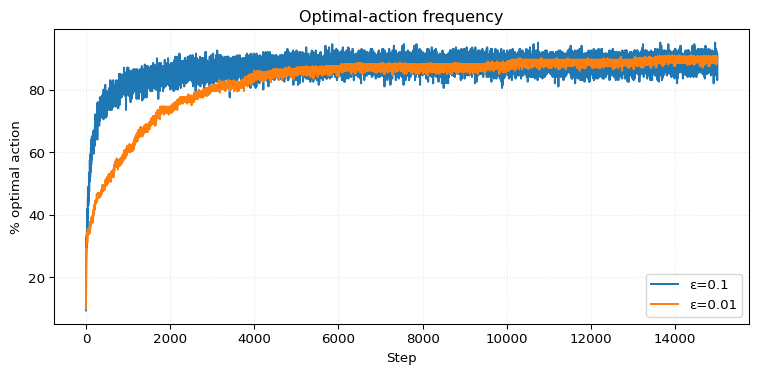
We can see that \(\varepsilon=0.01\) outperforms \(\varepsilon=0.1\) in average reward around step \(2000\). However, achieving a higher percentage of optimal actions takes more than \(10,000\) steps. It’s actually quite interesting that achieving a higher percentage of optimal actions takes significantly longer.

Now, let’s consider the long-term behaviour. In the limit, we can assume both methods have near-perfect \(Q\)-values and the only reason they select non-optimal actions is due to their \(\varepsilon\)-softness.

This makes calculating the optimal action probability quite easy. \[ \mathrm{Pr}(\text{optimal action}) = (1-\varepsilon) + \varepsilon \frac{1}{10} = 1 - 0.9 \varepsilon \]

So for \(\varepsilon=0.1\) this probability is \(0.91\), and for \(\varepsilon=0.01\) this is \(0.991\).

Now the average reward is trickier to compute. It can be done, but it’s quite messy and we’re here to learn reinforcement learning so we don’t need to figure out perfect analytical solutions anymore. Luckily, we get this value directly from the book

It [greedy algorithm] achieved a reward-per-step of only about \(1\), compared with the best possible of about \(1.55\) on this testbed (Sutton and Barto 2018, 29).

Great—they’ve done the work for us. Selecting the optimal action gives an average reward of \(1.55\). Selecting a random action has an average reward of \(0\) because it’s basically drawing a sample from a normal distribution with mean \(0\). That gives:

\[ \mathbb{E}[R_t] = (1-\varepsilon) 1.55 + \varepsilon 0 = 1.55 (1-\varepsilon) \]

This results in \(1.40\) for \(\varepsilon = 0.1\) and \(1.53\) for \(\varepsilon = 0.01\).

2.4 Incremental Implementation

The sample average can be updated incrementally using: \[ Q_{n+1} = Q_n + \frac{1}{n}[R_n - Q_n]. \tag{2.1}\]

This is an instance of a general pattern that is central to reinforcement learning: \[ \text{NewEstimate} \gets \text{OldEstimate} + \text{StepSize} \Big[\overbrace{ \text{Target} - \text{OldEstimate} }^\text{error} \Big] \]

I especially like how nice it looks in python. In value-based algorithms, this typically corresponds to the following line of code:

Q[action] += α * (reward - Q[action])

2.5 Tracking a Nonstationary Problem

To avoid the learning rate decreasing over time—at the cost of convergence—we can use a constant step size \(\alpha \in (0,1]\). \[ Q_{n+1} := Q_n + \alpha \Big[ R_n - Q_n \Big], \tag{2.2}\]

for \(n \geq 1\) and \(Q_1\) is our given initial estimate.

This can be phrased as a recurrence relation of the form \(Q_n = \sum_{i=0}^n \gamma^{n-i} r_i\), as discussed in the appendix Section 2.11.9: We add \(Q_0\) and \(R_0\). Then, Equation 2.2 is equivalent to: \[ Q_{n+1} = \alpha R_n + (1 - \alpha) Q_n \quad \text{and} \quad Q_0 = 0, \tag{2.3}\]

This is a recurrence relation of the form Equation 2.18 and thus has the explicit form \[ Q_{n+1} = \sum_{i=0}^n (1 - \alpha)^{n-i} \alpha R_{i} \]

Substituting \(R_0 = \frac{Q_1}{\alpha}\)—so that \(Q_1\) becomes our arbitrary initial value—yields the form used by Sutton and Barto: \[ Q_{n+1} = (1-\alpha)^n Q_1 + \sum_{i=1}^n \alpha (1 - \alpha)^{n-i} R_i \tag{2.4}\]

This is a weighted average of the random variables involved, as the weights sum to 1. The sum of the weights for the \(R_i\) is (using the geometric series identity Equation 2.14): \[ \begin{split} \sum_{i=1}^n \alpha (1- \alpha)^{n-i} &= \alpha \sum_{i=o}^{n-1}(1-\alpha)^i \\ &= \alpha \frac{1 - (1-\alpha)^n}{\alpha}\\ &= 1 - (1 - \alpha)^n. \end{split} \]

Thus, the total weight sums to 1: \[ \begin{split} (1-\alpha)^n + \sum_{i=1}^n \alpha (1 - \alpha)^{n-i} &= 1 \end{split} \]

The \(Q_n\) are estimators for the true action value \(q_*\). And depending on how we determine the \(Q_n\), they have different qualities. We note that the \(R_i\) are IID with mean \(q_*\) and variance \(\sigma^2\). (I refer to the appendix Section 2.11 for more information about all the new terms appearing all of a sudden, as this has gotten quite a bit more technical)

If \(Q_n\)​ is the sample average, the estimator is unbiased, that is \[ \mathbb{E}[Q_n] = q_* \quad \text{for all } n \in \mathbb{N}. \] Which is easy to show. Its mean squared error \(\mathrm{MSE}(Q_n) := \mathbb{E}[(Q_n - q_*)^2]\) is decreasing (Lemma 2.4): \[ \mathrm{MSE}(Q_n) = \frac{\sigma^2}{n}. \]

If the \(Q_n\) are calculated using a constant step size, they are biased (there is always a small dependency on \(Q_1\)): \[ \begin{split} \mathbb{E}[Q_{n+1}] &= (1-\alpha)^n Q_1 + q\sum_{i=1}^n \alpha (1 - \alpha)^{n-i} \\ &= (1-\alpha)^n Q_1 + q (1 - (1 - \alpha)^n) \end{split} \tag{2.5}\]

And even though they are asymptotically unbiased, i.e., \(\lim_{n\to\infty} \mathbb{E}[Q_{n}] = q\), their mean squared error is bounded away from zero (Lemma 2.5): \[ \mathrm{MSE}(Q_n) > \sigma^2 \frac{\alpha}{2-\alpha}. \]

It’s hard for me to translate these stochastic results in statistic behaviour, but I think that means that constant step size will end up wiggling around the true value.

Let’s define the constant step size agent to compare it with the sample average method later.

# === the constant step bandit agent ===
class ConstantStepBanditAgent:
    def __init__(self, Q1, α, ε, seed=None):
        self.rng = np.random.default_rng(seed)
        self.num_actions = len(Q1)
        self.Q1 = Q1
        self.α = α
        self.ε = ε
        self.reset()

    def reset(self):
        self.Q = self.Q1.copy()

    def act(self, bandit):
        # ε-greedy action selection
        if self.rng.random() < self.ε:
            action = self.rng.integers(self.num_actions)
        else:
            action = np.argmax(self.Q)

        # take action
        reward = bandit.pull_arm(action)

        # update value estimate
        self.Q[action] += self.α * (reward - self.Q[action])

        return (action, reward)

Exercise 2.4 If the step-size parameters, \(\alpha_n\), are not constant, then the estimate \(Q_n\) is a weighted average of previously received rewards with a weighting different from that given by Equation 2.4. What is the weighting on each prior reward for the general case, analogous to Equation 2.4, in terms of the sequence of step-size parameters.

Solution 2.4. The update rule for non-constant step size has \(\alpha_n\) depending on the step. \[ Q_{n+1} = Q_n + \alpha_n \Big[ R_n - Q_n \Big] \tag{2.6}\]

In this case the weighted average is given by \[ Q_{n+1} = \left( \prod_{j=1}^n 1-\alpha_j \right) Q_1 + \sum_{i=1}^n \alpha_i \left( \prod_{j=i+1}^n 1 - \alpha_j \right) R_i \tag{2.7}\]

This explicit form can be verified inductively. For \(n=0\), we get \(Q_1\) on both sides.

For the induction step we have \[ \begin{split} Q_{n+1} &= Q_n + \alpha_n \Big[ R_n - Q_n \Big] \\ &= \alpha_n R_n + (1 - \alpha_n) Q_n \\ &= \alpha_n R_n + (1 - \alpha_n) \Big[ \left( \prod_{j=1}^{n-1} 1-\alpha_j \right) Q_1 + \sum_{i=1}^{n-1} \alpha_i \left( \prod_{j=i+1}^{n-1} 1 - \alpha_j \right) R_i \Big] \\ &= \left( \prod_{j=1}^n 1-\alpha_j \right) Q_1 + \sum_{i=1}^n \alpha_i \left( \prod_{j=i+1}^n 1 - \alpha_j \right) R_i \end{split} \]

We also note that in this general setting, Equation 2.7 is still a weighted average. We could prove it by induction or use a little trick. If we set \(Q_1 = 1\) and \(R_n = 1\) for all \(n\) in the recurrence relation Equation 2.6 we see that each \(Q_n = 1\). If we do the same in the explicit formula Equation 2.7 we see that each \(Q_n\) is equal to the sum of the weights. Therefore, the weights sum up to \(1\).

Exercise 2.5 Design and conduct an experiment to demonstrate the difficulties that sample-average methods have for nonstationary problems. Use a modified version of the 10-armed testbed in which all the \(q_\star(a)\) start out equal and then take independent random walks (say by adding a normally distributed increment with mean zero and standard deviation 0.01 to all the \(q_\star(a)\) on each step). Prepare plots like Figure Figure 2.1 for an action-value method using sample averages, incrementally computed, and another action-value method using a constant step-size parameter, \(\alpha = 0.1\). Use \(\epsilon = 0.1\) and longer runs, say of 10,000 steps

Solution 2.5. Alright, let’s do a little experiment, just as they told us.

# === battle between sample average and constant step ===
config = Config(
    bandit_setup_mu=0,
    bandit_setup_sd=0,
    bandit_value_drift=True,
    bandit_value_drift_mu=0,
    bandit_value_drift_sd=0.01,
    exp_steps=10_000,
    exp_runs=100,
)

agent0 = SampleAverageBanditAgent(Q1=np.zeros(config.bandit_num_arms, dtype=float), ε=0.1, seed=config.exp_seed)
agent1 = ConstantStepBanditAgent(
    Q1=np.zeros(config.bandit_num_arms, dtype=float), α=0.1, ε=0.1, seed=config.exp_seed
)
agents = [agent0, agent1]

avg_rwd, opt_pct = bandit_experiment(
    agents,
    config
)

labels = ["sample averages (ε=0.1)", "constant step-size (α=0.1, ε=0.1)"]
plot_average_reward(avg_rwd, labels=labels)
plt.tight_layout()
plt.show()

plot_optimal_action_percent(opt_pct, labels=labels)
plt.tight_layout()
plt.show()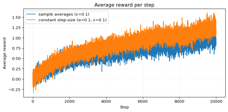

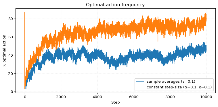
Not surprisingly, we can see how much the sample average agent struggles to keep up. For longer episode lengths, the problem only gets worse. Eventually, it will be completely out of touch with the world, like an old man unable to keep up with the times.

However, it remains unclear exactly how rapidly the sample average method will deteriorate to an unacceptable level. The results from the final exercise of this chapter (Exercise 2.11) indicate that this deterioration may take a significant number of steps.

2.6 Optimistic Initial Values

We later need the following figure comparing an optimistic greedy agent and a realistic \(\varepsilon\)-greedy agent.

# === realism vs optimism ===
config = Config(
    exp_steps=1_000,
    exp_runs=1_000
)
agent_optimistic_greedy = ConstantStepBanditAgent(
    Q1=np.full(config.bandit_num_arms, 5.0, dtype=float), α=0.1, ε=0.0, seed=config.exp_seed
)
agent_realistic_ε_greedy = ConstantStepBanditAgent(
    Q1=np.zeros(config.bandit_num_arms, dtype=float), α=0.1, ε=0.1, seed=config.exp_seed
)

agents = [agent_optimistic_greedy, agent_realistic_ε_greedy]
avg_rwd, opt_pct = bandit_experiment(
    agents,
    config
)

labels = [
    "optimistic,greedy (Q1=5, ε=0, α=0.1)",
    "realistic,ε-greedy (Q1=0, ε=0.1, α=0.1)",
]
plot_optimal_action_percent(opt_pct, labels=labels)
plt.tight_layout()
plt.show()

Figure 2.2: This is like Figure 2.3 (Sutton and Barto 2018): the effect of optimistic initial action-value estimates.

Exercise 2.6 (Mysterious Spikes) The results shown in Figure 2.2 should be quite reliable because they are averages over 2000 individual, randomly chosen 10-armed bandit tasks. Why, then, are there oscillations and spikes in the early part of the curve for the optimistic method? In other words, what might make this method perform particularly better or worse, on average, on particular early steps?

Solution 2.6. We have the hard-earned luxury that we can zoom in on Figure 2.2:

# === realism vs optimism zoomed in ===
config = Config(
    exp_steps=30,
    exp_runs=5_000,
)
agent_optimistic_greedy = ConstantStepBanditAgent(
    Q1=np.full(config.bandit_num_arms, 5.0, dtype=float), α=0.1, ε=0.0, seed=config.exp_seed
)
agent_realistic_ε_greedy = ConstantStepBanditAgent(
    Q1=np.zeros(config.bandit_num_arms, dtype=float), α=0.1, ε=0.1, seed=config.exp_seed
)

agents = [agent_optimistic_greedy, agent_realistic_ε_greedy]
avg_rwd, opt_pct = bandit_experiment(
    agents,
    config
)

labels = [
    "optimistic,greedy (Q1=5, ε=0, α=0.1)",
    "realistic,ε-greedy (Q1=0, ε=0.1, α=0.1)",
]
plot_optimal_action_percent(opt_pct, labels=labels)
plt.tight_layout()
plt.show()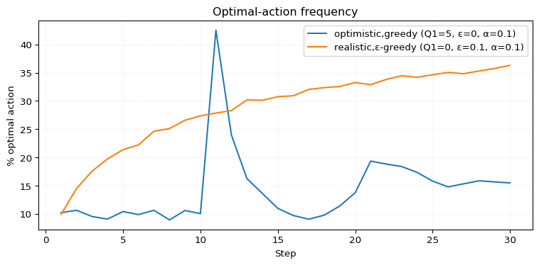

The spike occurs at step 11. Essentially, the optimistic method samples all actions once (poor performance), and then selects the action with the best result (good performance, with a success rate of over 40%). However, regardless of the outcome (which likely pales in comparison to the current Q-values, which are still likely greater than 4), the method returns to exploring all 10 actions again. This leads to poor performance once more. Around step 22, there is another spike for similar reasons, but this time smaller and more spread out.

Exercise 2.7 (Unbiased Constant-Step-Size Trick) In most of this chapter we have used sample averages to estimate action values because sample averages do not produce the initial bias that constant step sizes do (see the analysis leading to (2.6)). However, sample averages are not a completely satisfactory solution because they may perform poorly on nonstationary problems. Is it possible to avoid the bias of onstant step sizes while retaining their advantages on nonstationary problems? One way is to use a step size of \[ \beta_n := \alpha / \bar{o}_n \] to process the \(n\)-th reward for a particular action, where \(\alpha > 0\) is a conventional constant step size, and \(\bar{o}_n\) is a trace of one that starts at \(0\): \[ \bar{o}_n := \bar{o}_{n-1} + \alpha (1 - \bar{o}_{n-1}), \text{ for } n \geq 1, \text{ with } \bar{o}_0 := 0 \] Carry out an analyises like that in Equation 2.4 to show that \(Q_n\) is an exponential recency-weighted average without initial bias.

Solution 2.7. My first question when I saw this was, “What’s up with that strange name \(\bar{o}_n\)?”” I guess it could be something like “the weighted average of ones”, maybe? Well, whatever. Let’s crack on.

When we rewrite \(\bar{o}_{n+1}\) as a recurrence relation for \(\frac{\bar{o}_{n+1}}{\alpha}\) \[ \frac{\bar{o}_{n+1}}{\alpha} = 1 + (1 - \alpha) \frac{\bar{o}_n}{\alpha} \] we see that it is just the recurrence relation for a geometric series as in Equation 2.13 for \(\gamma = 1-\alpha\). Thus we get \[ \bar{o}_n = \alpha\sum_{i=0}^{n-1} (1 - \alpha)^{i} = 1 - (1-\alpha)^n \] and \(\beta_n = \frac{\alpha}{1-(1-\alpha)^n}\)

(btw. this is such a complicated way to define \(\beta_n\) and I don’t understand why actually.)

In particular we have that \(\beta_1 = 1\), which makes the influence of \(Q_1\) disappears after the first reward \(R_1\) is received: \(Q_2 = Q_1 + 1 [ R_1 - Q_1] = R_1\). Great!

Scaling the \(\alpha\) by the \(\bar{o}_n\) has an additional nicer effect. I don’t quite understand how, but we can calculate it.

From Exercise 2.4 we know \[ Q_{n+1} = Q_1 \prod_{j=1}^n (1-\beta_j) + \sum_{i=1}^n R_i \beta_i \prod_{j=i+1}^n (1- \beta_j ) \]

There is a nice form for these products \[ \prod_{j=i}^n (1 - \beta_j) = (1-\alpha)^{n-j+1} \frac{\bar{o}_{i-1}}{\bar{o}_n} \]

since they are telescoping using \[ \begin{split} 1- \beta_j &= 1 - \frac{\alpha}{\bar{o}_j} = \frac{\bar{o}_j - \alpha}{\bar{o}_j}\\ &= \frac{\alpha + (1-\alpha) \bar{o}_{j-1}}{\bar{o}_j} = (1-\alpha)\frac{\bar{o}_{j-1}}{\bar{o}_j}. \end{split} \]

This gives the following closed form for \(Q_{n+1}\) \[ Q_{n+1} = \frac{\alpha}{1 - (1-\alpha)^n}\sum_{i=1}^n R_i (1-\alpha)^{n-i} \]

We can see that the weight given to any reward \(R_i\)​ decreases exponentially.

2.7 Upper-Confidence-Bound Action Selection

We have the opportunity to introduce a new agent here. The update rule remains the same (I assume sample average), but the action selection is more informed compared to \(\varepsilon\)-greedy algorithms.

\[ A_t := \mathrm{argmax}_a \left[ Q_t(a) + c \sqrt{ \frac{\ln t}{N_t(a)} }\right] \]

where \(N_t(a)\) is the number of times that action has been selected, c > 0 controls the exploration (similar to \(\varepsilon\)).

If an action has not been selected even once, i.e., \(N_t(a)=0\), then \(a\) is considered to be a maximizing action. (In our case, this means that in the first few steps, all actions have to be selected once, and only after that does the UCB-based action selection kick in.)

By the way, I have no idea where the UCB formulation comes from, but at least it looks fancy (and reasonable), and we can implement it:

# === the ucb bandit agent ===
class UcbBanditAgent:
    def __init__(self, num_actions, c, seed=None):
        self.num_actions = num_actions
        self.c = c  # exploration parameter
        self.reset()
        self.rng = np.random.default_rng(seed)

    def reset(self):
        self.t = 0
        self.Q = np.zeros(self.num_actions, dtype=float)
        self.counts = np.zeros(self.num_actions, dtype=int)

    def act(self, bandit):
        self.t += 1

        # upper-Confidence-Bound Action Selection
        if self.t <= self.num_actions:
            # if not all actions have been tried yet, select an untried action
            action = self._choose_untaken_action()
        else:
            # calculate UCB values for each action
            ucb_values = self.Q + self.c * np.sqrt(np.log(self.t) / (self.counts))
            # select the action with the highest UCB value
            action = np.argmax(ucb_values)

        # take action and observe the reward
        reward = bandit.pull_arm(action)

        # update count and value estimate
        self.counts[action] += 1
        self.Q[action] += (reward - self.Q[action]) / self.counts[action]

        return (action, reward)

    def _choose_untaken_action(self):
        return self.rng.choice(np.where(self.counts == 0)[0])

Let’s recreate the figure illustrating UCB action selection performance, which we’ll need for the next exercise.

# === ucb agent performance ===
config = Config(
    exp_steps=1_000,
    exp_runs=1_000,
)
agent_ucb = UcbBanditAgent(num_actions=config.bandit_num_arms, c=2, seed=config.exp_seed)
agent_ε_greedy = SampleAverageBanditAgent(
    Q1=np.zeros(config.bandit_num_arms, dtype=float), ε=0.1, seed=config.exp_seed
)

agents = [agent_ucb, agent_ε_greedy]

avg_rwd, opt_pct = bandit_experiment(
    agents,
    config
)

labels = [
    "ucb (c=2, α=0.1)",
    "ε-greedy (ε=0.1, α=0.1)",
]
plot_optimal_action_percent(opt_pct, labels=labels)
plt.tight_layout()
plt.show()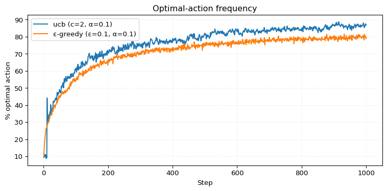

Figure 2.3: This is like Figure 2.4 (Sutton and Barto 2018): average performance of UCB action selection.

Exercise 2.8 (UCB Spikes) In Figure 2.3 the UCB algorithm shows a distinct spike in performance on the 11th step. Why is this? Note that for your answer to be fully satisfactory it must explain both why the reward increases on the 11th step and why it decreases on the subsequent steps. Hint: if \(c = 1\), then the spike is less prominent.

Solution 2.8. I think the answer is similar to the answer to Exercise 2.6. The first \(10\) steps the UCB algorithm tries out all actions. Then on step \(11\) it will select the one that scored highest, which is quite a decent strategy. But then because of the \(N_t​(a)\) in the denominator it is back to exploring.

2.8 Gradient Bandit Algorithms

This introduces a novel method that is not value-based; instead, it directly aims to select the best actions. The agent maintains numerical preferences, denoted by \(H_t​(a)\), rather than estimates of the action values.

For action selection, gradient bandit uses the softmax distribution: \[ \pi_t(a) = \frac{e^{H_t(a)}}{\sum_{b=1}^k e^{H_t(b)}}. \tag{2.8}\]

Shifting all preferences by a constant \(C\) doesn’t affect \(\pi_t(a)\): \[ \pi_t(a) = \frac{e^{H_t(a)}}{\sum_{b=1}^k e^{H_t(b)}} = \frac{e^Ce^{H_t(a)}}{\sum_{b=1}^k e^Ce^{H_t(b)}} = \frac{e^{H_t(a)+C}}{\sum_{b=1}^k e^{H_t(b)+C}} \]

For learning, gradient bandit uses the following rule: \[ \begin{split} H_{t+1}(a) &:= H_t(a) + \alpha (R_t - \bar{R}_t) (\mathbb{I}_{a = A_t} - \pi_t(a)) \end{split} \tag{2.9}\]

Now, let’s implement this gradient bandit algorithm:

# === the gradient agent ===
class GradientBanditAgent:
    def __init__(self, H1, α, baseline=True, seed=None):
        self.num_actions = len(H1) 
        self.α = α 
        self.H1 = np.asarray(H1, dtype=np.float64)  # initial preferences
        self.baseline = baseline # apply average reward baseline
        self.reset()
        self.rng = np.random.default_rng(seed)

    def reset(self):
        self.H = self.H1.copy()  
        self.avg_reward = 0 
        self.t = 0  # step count

    def act(self, bandit):
        self.t += 1

        # select action using softmax
        action_probs = GradientBanditAgent.softmax(self.H)
        action = self.rng.choice(self.num_actions, p=action_probs)

        # take action and observe the reward
        reward = bandit.pull_arm(action)

        # update average reward
        if self.baseline:
            self.avg_reward += (reward - self.avg_reward) / self.t

        # update action preferences
        advantage = reward - self.avg_reward # avg_reward = 0 if baseline = false
        one_hot_action = np.eye(self.num_actions)[action]
        self.H += self.α * advantage * (one_hot_action - action_probs)

        return action, reward

    @staticmethod
    def softmax(x):
        # shift vector by max(x) to avoid hughe numbers.
        # This is basically using the fact that softmax(x) = softmax(x + C)
        exp_x = np.exp(x - np.max(x))
        return exp_x / np.sum(exp_x)

Sutton and Barto (Sutton and Barto 2018, 37) emphasize the importance of the baseline \(\bar{R}_t\)​ in the update forumla and show that performance drops without it. In the derivation of the update as a form of stochastic gradient ascent, the baseline can be chosen arbitrarily (see Section 2.8.1). Whether or not a baseline is used, the resulting updates are unbiased estimators of the gradient. I assume, the baseline serves to reduce the variance of the estimator, although I have no idea about the maths behind it.

Here we recreat Figure 2.5 (Sutton and Barto 2018), which shows how drastically the running average baseline can improve performance.

# === gradient bandit performance ===
config = Config(
    exp_steps=1_000,
    exp_runs=50,
    bandit_setup_mu=4,
)

alphas = [0.1, 0.4]
agents = [GradientBanditAgent(H1=np.zeros(config.bandit_num_arms), α=α, seed=config.exp_seed) for α in alphas] + [GradientBanditAgent(H1=np.zeros(config.bandit_num_arms), α=α, baseline=False, seed=config.exp_seed) for α in alphas]

avg_rwd, opt_pct = bandit_experiment(
    agents,
    config
)

labels = [f"α = {α}, with baseline" for α in alphas] + [f"α = {α}, without baseline" for α in alphas]
plot_optimal_action_percent(opt_pct, labels=labels)
plt.tight_layout()
plt.show()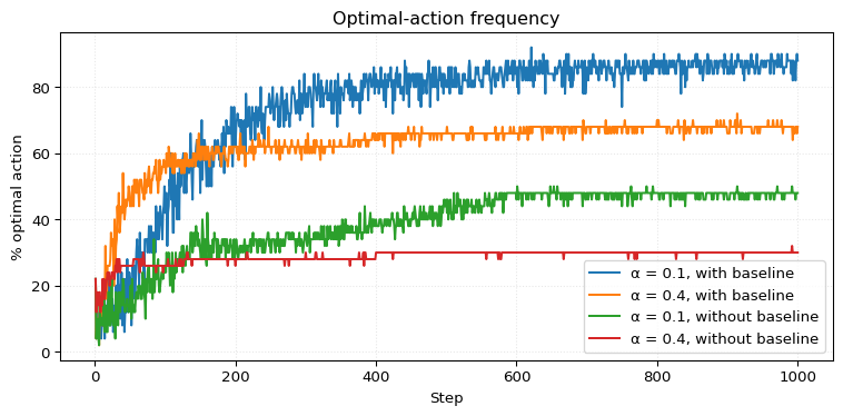

Figure 2.4: This is like Figure 2.5 (Sutton and Barto 2018): average performance of the gradient bandit algorithm with and without a reward baseline on the 10-armed testbed when the \(q_*(a)\) are chosen to be near \(+4\) rather than near zero. (we averaged over 50 runs because it gives this cool jaggedy looking graph)

Exercise 2.9 Show that in the case of two actions, the soft-max distribution is the same as that given by the logistic, or sigmoid, function often used in statistics and artificial neural networks.

Solution 2.9. The logistic function is defined as \[ \sigma(x) := \frac{1}{1 + e^{-x}} = \frac{e^x}{1+e^x}. \] If we map the two preferences \(H(a_1), H(a_2)\) to a single value \(\Delta = H(a_1) - H(a_2)\) then \[ \pi(a_1) = \frac{e^{H(a_1)}}{e^{H(a_1)} + e^{H(a_2)}} = \frac{e^{H(a_1)-H(a_2)}}{e^{H(a_1)-H(a_2)} + 1} = \sigma(\Delta) \] and similarly \[ \pi(a_2) = \sigma(-\Delta). \]

2.8.1 the bandit gradient algorithm as stochastic gradient ascent

This next subsection is devoted to the (I imagine) infamous brown box (Sutton and Barto 2018, 38–40), which marks a significant leap in theoretical complexity. It shows how the update rule arises as a form of stochastic gradient ascent.

We’ll retrace their steps as a self-contained argument and flag two subtle points: the role of the baseline and the randomness in the preference vector.

1. quick recap of gradient ascent

Let \(f \colon \mathbb{R}^n \to \mathbb{R}\) be a differentiable function. We want to produce points \(\mathbf{x}_0, \mathbf{x}_1, \dots\) that maximise \(f\). Gradient ascent updates the current point \(\mathbf{x}^{(t)}\) in the direction of the gradient: \[ \mathbf{x}^{(t+1)} = \mathbf{x}^{(t)} + \alpha \; \nabla f(\mathbf{x})\big|_{\mathbf{x}^{(t)}} \] where \(\alpha > 0\) is the step size.

In one dimension, this becomes: \[ x_i^{(t+1)} = x_i^{(t)} + \alpha \; \frac{\partial f(\mathbf{x})}{\partial x_i}\bigg|_{x_i^{(t)}} \]

In stochastic gradient ascent, we aim to maximise the expected value of a random vector \(\mathbf{R}\) (a vector whose values are random variables), whose distribution depends on a parameter vector \(\mathbf{x}\). That is, the underlying probability space \((\Omega, \mathrm{Pr}_{\mathbf{x}})\) is parameterised by \(\mathbf{x}\). Here \(f\) is \(\mathbb{E}_{\mathbf{x}}[\mathbf{R}]\) where we have explicitly indicated the dependence of the expected value on \(\mathbf{x}\). So this is still a deterministic gradient ascent step—although the true gradient is unknown to the algorithm and must later be estimated via sampling: \[ \mathbf{x}^{(t+1)} = \mathbf{x}^{(t)} + \alpha \cdot \nabla \mathbb{E}_{\mathbf{x}}[\mathbf{R}]\big|_{\mathbf{x}^{(t)}} \]

Our goal is to cast the gradient bandit update in this framework.

2. setting up the problem

In the gradient bandit algorithm, the parameters we adjust are the action preferences \(H_t​(a)\). These determine the policy via the softmax distribution: \[ \pi_H(a) = \frac{e^{H(a)}}{\sum_{b \in \mathcal{A}} e^{H(b)}} \]

This shows how our parameter \(H\) determines the probability space: it determines the probability distribution for \(A_t\) \(\pi_{H_t}(a) := \mathrm{Pr}_{H_t}(A_t = a)\) the probabilities for rewards given an action are determined by the system and independent of the parameters \(q_*(a) := \mathbb{E}[R_t \mid A_t = a]\).

With this set-up, it is clear how \(\mathbb{E}_{H_t}[R_t]\) is a function on \(H_t\) \[ \begin{split} \mathbb{E}_{H_t}[R_t] &= \sum_{b} \mathrm{Pr}_{H_t}(A_t = b) \cdot \mathbb{E}[R_t \mid A_t = b] \\ &= \sum_{b} \pi_{H_t}(b) q_*(b) \end{split} \] (if you are unsure about this, check Theorem 2.4).

In this context, each action \(a\in\mathcal{A}\) corresponds to a coordinate in our parameter vector \(H\), so the gradient update in one dimension \(a \in \mathcal{A}\) becomes: \[ H_{t+1}(a) = H_t(a) + \alpha \frac{\partial \mathbf{E}[R_t]}{\partial H(a)}\bigg|_{H_t(a)} \tag{2.10}\]

3. calculating the gradient

Now look at the row of the gradient for \(a \in \mathcal{A}\): \[ \begin{split} \frac{\partial \mathbb{E}_{H}[R_t]}{\partial H(a)}\Bigg|_{H_t(a)} &= \sum_{b} q_*(b) \cdot \frac{\partial \pi_{H}(b)}{\partial H(a)}\Bigg|_{H_t(a)} \\ &= \sum_{b} (q_*(b) - B_t) \cdot \frac{\partial \pi_{H}(b)}{\partial H(a)}\Bigg|_{H_t(a)} \end{split} \] We could add here any scalar (called the baseline) as \(\sum_b \pi_H(b) = 1\) and thus \(\sum_{b} \frac{\partial \pi_{H}(b)}{\partial H(a)}\Big|_{H'(a)} = 0\). Note that for this argument to work \(B_t\) cannot depend on \(b\).

To simplify that further we use the softmax derivative, (which is derived in Sutton and Barto): \[ \frac{\partial \pi_{H}(b)}{\partial H(a)}\Bigg|_{H_t(a)} = \pi_{H_t}(b) (\mathbb{I}_{a = b} - \pi_{H_t}(a)) \]

So we have \[ \begin{split} \frac{\partial \mathbb{E}_{H}[R_t]}{\partial H(a)}\Bigg|_{H_t(a)} &= \sum_{b} (q_*(b) - B_t) \cdot (\mathbb{I}_{a = b} - \pi_{H_t}(a)) \pi_{H_t}(b) \\ &= \mathbb{E}_{H_t}[(q_*(A_t)- B_t) (\mathbb{I}_{a = A_t} - \pi_{H_t(a)})] \\ &= \mathbb{E}_{H_t}[ (R_t - B_t) (\mathbb{I}_{a = A_t} - \pi_{H_t(a)})]. \end{split} \] We get the second equality by applying the law of the unconscious statistician in reverse (Theorem 2.1), and yes the expression inside the expectation is all just a deterministic function of \(A_t\). In the final equality, we substituted \(R_t\) for \(q_*(A_t)\) using that \(q_*(A_t) = \mathbb{E}_{H_t}[R_t]\), and the law of iterated expectations justifies the substitution under the outer expectation.

Before going to the next step, you might want to check the plausibility of \[ \frac{\partial \mathbb{E}[R_t]}{\partial H(a)}\Bigg|_{H_t(a)} = \mathbb{E}_{H_t}[ (R_t - B_t) (\mathbb{I}_{a = A_t} - \pi_{H_t(a)})]. \tag{2.11}\] On the left we have basically a number, the value of the derivative at some point, and on the right we have an expected value with a parameter \(B_t\). So the parameter \(B_t\) must cancel out somehow. Which it does indeed, you can check this for yourself.

4. one-step update and baseline trade-off

By plugging Equation 2.11 into Equation 2.10 we get the deterministic gradient ascent update: \[ H_{t+1}(a) = H_t(a) + \alpha \mathbb{E}[ (R_t - B_t) (\mathbb{I}_{a = A_t} - \pi_{H_t(a)})] \]

Replacing the expectation by the single sample \(A_t, R_t\) yields the stochastic gradient update: \[ H_{t+1}(a) = H_t(a) + \alpha (R_t - B_t) (\mathbb{I}_{a = A_t} - \pi_{H_t(a)}) \tag{2.12}\]

To get Equation 2.9 we have to substitute \(\bar{R}_t\) for \(B_t\). Which requires some discussion first.

Sutton and Barto make clear that \(\bar{R}_t\) depend on \(R_t\):

\(\bar{R}_t\) is the average of all the rewards up through and including time \(t\) (Sutton and Barto 2018, 37).

If we use that in Equation 2.12 for \(B_t\) we are not using an unbiased estimator anymore. This is tightly coupled with the fact that when we introduced \(B_t\) we required it not to depend on \(b\) which does later play the role of \(A_t\), and \(\bar{R}_t\) depends on \(R_t\) which depends on \(A_t\).

Mostl likely there is a good reason for using \(\bar{R}_t\), but I don’t know the mathematical motivation. (As I said, maybe some variance reduction)

However I’m saying the derivation of their update formula is wrong¹ as they frame it as an unbiased estimator.

comment on the time parameter

We have keept the time parameter in the derivation to stick to the style of Sutton and Barto. We could have equally done the same derivation for \(H'\) (new) and \(H\) (old). However, conceptually keeping the time parameter is a bit shaky. Where does the \(H_t\) come from? If we think this through then \(H_t\) actually becomes part of the whole system (enviroment + agent) and thus is a random vector. And then it’s harder for me to think about how to analyse this to obtain the update formula. Once the update rule is fixed, we can then treat the entire system (agent and environment) as stochastic without any problems.

If correct or not Sutton-Barto derive this term for the gradient \[ \mathbb{E}\big[ (R_t - \bar{R}_t) (\mathbb{I}_{a = A_t} - \pi_{H_t}(a)) \big]. \] Which might look a bit fishy because maybe \(\mathbb{E}\big[ R_t - \bar{R}_t]\) is always \(0\). But it is usually not, because the policy \(\pi\) is not stationary, it get’s updated at every step and thus the policy’s evolution decouples the two expectations.

2.9 Associative Search (Contextual Bandits)

Exercise 2.10 Suppose you face a \(2\)-armed bandit task whose true action values change randomly from time step to time step. Specifically, suppose that, for any time step, the true values of actions \(1\) and \(2\) are respectively \(0.1\) and \(0.2\) with probability \(0.5\) (case A), and \(0.9\) and \(0.8\) with probability \(0.5\) (case B). If you are not able to tell which case you face at any step, what is the best expectation of success you can achieve and how should you behave to achieve it? Now suppose that on each step you are told whether you are facing case A or case B (although you still don’t know the true action values). This is an associative search task. What is the best expectation of success you can achieve in this task, and how should you behave to achieve it?

Solution 2.10. We are presented with two scenarios and the questions “What is the best strategy?” and “What is its expected reward?” for each scenario.

In the first scenario, we don’t know whether we are facing Case A or Case B at any given time step. The true values of the actions are as follows: \[ \begin{split} \mathbb{E}[R_t \mid A_t = 1] &= \mathrm{Pr}(\text{Case A}) \cdot 0.1 + \mathrm{Pr}(\text{Case B}) \cdot 0.9\\ &= 0.5 (0.1 + 0.9) = 0.5\\[3ex] \mathbb{E}[R_t \mid A_t = 2] &= \mathrm{Pr}(\text{Case A}) \cdot 0.2 + \mathrm{Pr}(\text{Case B}) \cdot 0.8\\ &= 0.5 (0.2 + 0.8) = 0.5 \end{split} \]

Since both actions have the same expected reward of 0.5, it does not matter which action is chosen. Thus, any algorithm is optimal and has an expected of 0.5.

In the second scenario, we know whether we are facing Case A or Case B. The expected reward under the optimal strategy, which always chooses the action with the highest expected value, is: \[ \mathbb{E}_{\pi_*}[ R_t ] = \overbrace{0.5 \cdot 0.2}^{\text{case A}} + \overbrace{0.5 \cdot 0.9}^{\text{case B}} = 0.55 \]

To achieve this expected reward, we need to keep track of the two bandit problems separately and maximise their rewards. How to do this approximately is the topic of the whole chapter.

2.10 Summary

Exercise 2.11 Make a figure analogous to Figure 2.6 for the nonstationary case outlined in Exercise 2.5. Include the constant-step-size \(\varepsilon\)-greedy algorithm with \(\alpha\)= 0.1. Use runs of 200,000 steps and, as a performance measure for each algorithm and parameter setting, use the average reward over the last 100,000 steps.

Solution 2.11. That last exercise is a banger to finish with. There’s a lot going on here. I’ll explain what was difficult for me at the end, but let’s start with what I actually did and what we can see in the graph.

I ran a parameter sweep for four different bandit agents over 200 episodes of 300,000 steps each. For each episode, I only looked at the average reward over the last 50,000 steps to measure steady-state performance.

# === Parameter sweep for nonstationary bandit ===
"""
We compare 4 bandit agents:
0 - ε-greedy sample-average, parameter = ε
1 - ε-greedy constant α = 0.1, parameter = ε
2 - Gradient ascent with baseline, parameter = α
3 - Gradient ascent no baseline, parameter = α
"""
from functools import partial
from matplotlib.ticker import FuncFormatter

import numpy as np
import matplotlib.pyplot as plt

# custom import
from scripts.parameter_study.episode_mean import episode_mean

# --- Global config
CONFIG = dict(
    seed=1000000,
    num_arms=10,
    steps=300_000,
    keep=50_000,
    runs=200,
    q_0=10,
    drift_sd=0.1,
)

AGENTS = {
    "ε in ε-greedy (sample-avg)": dict(
        id=0,
        x_name="ε",
        x_vals=[2**-k for k in (12, 9, 6, 3, 1, 0)],
        fixed=dict(),
    ),
    "ε in ε-greedy (α = 0.1)": dict(
        id=1,
        x_name="ε",
        x_vals=[2**-k for k in (12, 9, 6, 3, 1, 0)],
        fixed=dict(α=0.1),
    ),
    "α in gradient ascent": dict(
        id=2,
        x_name="α",
        x_vals=[2**-k for k in (20, 18, 14, 9, 6, 3, 1)],
        fixed=dict(),
    ),
    "α in gradient ascent (no base)": dict(
        id=3,
        x_name="α",
        x_vals=[2**-k for k in (20, 18, 14, 9, 6, 3, 1)],
        fixed=dict(),
    ),
}


# --- Experiment helper
def evaluate(agent_type: int, **kwargs) -> float:
    """Mean reward over the last *keep* steps averaged across *runs* runs."""
    args = {**CONFIG, **kwargs}
    rng = np.random.default_rng(args["seed"])
    seeds = rng.integers(0, 2_000_000, size=args["runs"])

    rewards = [
        episode_mean(
            agent_type,
            args["num_arms"],
            args["steps"],
            args["keep"],
            args["q_0"],
            1,  # bandit_action_sd
            0,  # drift_mu
            args["drift_sd"],
            seed,
            kwargs.get("ε", 0.1),
            kwargs.get("α", 0.1),
        )
        for seed in seeds
    ]
    return float(np.mean(rewards))


# --- run the sweeps
results = {}
for label, spec in AGENTS.items():
    run = partial(evaluate, spec["id"], **spec["fixed"])
    results[label] = [run(**{spec["x_name"]: x}) for x in spec["x_vals"]]

# --- plot
fig, ax = plt.subplots(figsize=(10, 6))

markers = ["^", "o", "s", "*"]  # one per agent
for (label, spec), marker in zip(AGENTS.items(), markers):
    ax.plot(
        spec["x_vals"],
        results[label],
        marker=marker,
        label=label,
    )

ax.set_xscale("log", base=2)
ax.set_xlabel("Exploration / step-size (log scale)")
ax.set_ylabel(
    f"Average reward for the last {CONFIG['keep']:,} steps ({CONFIG['steps']:,} steps total)"
)
ax.set_title(f"Average reward (mean of {CONFIG['runs']} runs)")
ax.grid(True, which="both", linewidth=0.5)

ax.xaxis.set_major_formatter(
    FuncFormatter(lambda x, _: f"1/{int(1/x)}" if x < 1 else str(int(x)))
)

ax.legend()
fig.tight_layout()

plt.show()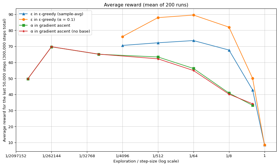

Parameter sweep for a non-stationary bandit, similar to Figure 2.6 (Sutton and Barto 2018). The plot displays the average reward of the last 50,000 steps of a 300,000-step episode, averaged over 200 runs. The bandit was initialized with action-value means set to 10, which drifted according to a normal distribution with a standard deviation of 0.1 at each step. The standard deviation of the reward noise was 1.

The agents I tested were:

• \(\varepsilon\)-greedy with sample-average action values, sweeping over \(\varepsilon\)
• \(\varepsilon\)-greedy with constant step-size (α = 0.1), also sweeping \(\varepsilon\)
• gradient ascent with a sample-average baseline, sweeping \(\alpha\)
• gradient ascent with no baseline, again sweeping \(\alpha\)

To encourage adaptability, I changed the drift to 0.1.

Let’s go through some observations:

1. constant step-size ε-greedy outperforms the others. Not that surprising.
2. gradient ascent underperforms. That surprised me. I’d assumed the gradient method would be a good fit for a drifting environment. However, it does worse than the sample-average ε-greedy.
3. small α performs best for gradient ascent. This one I don’t have a great explanation for, as very small step sizes typically result in slow learning.
4. also, the baseline doesn’t matter for verly low α. Again no clue.
5. sample-average ε-greedy agent is better than I expected. I thought that, with that many steps, it wouldn’t be able to keep up with the changing environment.
6. random Behaviour for ε = 1. The ε-greedy agents with ε = 1 behaves randomly, as expected. Both agents achieve a reward of 10, which is consistent with random action selection.

So, this figure raises quite a few questions I can’t yet answer. I think that makes this execrise really good. And maybe in the future I will be able to provide more insights about these findings.

This was a lot of work. Running 200 episodes at 300,000 steps each is way too slow in pure Python. I had to offload the inner loop into a separate file and used Numba to JIT-compile it, basically rewriting all the algorithms used in this experiment. That’s also why I don’t want to spend more time trying out gradient ascent with a constant-step baseline. Additionally, I can’t guarantee that there isn’t some subtle bug in the code for the main loop, as I didn’t really test all the algorithms.

2.11 appendix

Here are some more details on concepts that came up during this chapter.

2.11.1 distribution

Every random variable \(X\) has a distribution, denoted \(p_X\), which maps each possible value to its probability: \[ p_X(x) := \mathrm{Pr}(X = x). \]

Often, we say \(X\) is distributed according to \(f\) for a function \(f \colon \mathcal{X} \to [0,1]\), which means that \(f(x) = \mathrm{Pr}(X = x)\). We write this as: \[ X \sim f. \]

Two random variables \(X\) and \(Y\) have the same distribution if \(p_X = p_Y\).

The distribution of \(X\) turns \((\mathcal{X}, p_X)\) into a probability space, where \(p_X\) is called the pushforward measure.

2.11.2 independent and identically distributed random variables

A very important concept: IID. A collection of random variables \(X_1, \dots, X_n\) is independent and identically distributed (IID) if all random variables have the same probability distribution, and all are mutually independent.

Formally, this means:

• \(\mathrm{Pr}(X_i = x) = \mathrm{Pr}(X_j = x)\)
• \(\mathrm{Pr}(X_i = x,\, X_j = x') = \mathrm{Pr}(X_i = x) \cdot \mathrm{Pr}(X_j = x')\)

for all distinct indices \(i \neq j\).

2.11.3 lotus

The following theorem is widely known as the “law of the unconscious statistician”. It is fundamental in many calculations as it allows us to compute the expected value of functions of random variables by only knowing the distributions of the random variables.

Theorem 2.1 Let \(X \colon \Omega \to \mathcal{X}\) be a random variable, and let \(g \colon \mathcal{X} \to \mathbb{R}\) be a real-valued function on the result space.
Then the expected value of \(g\) with respect to the pushforward distribution \(p_X\) is the same as the expected value of the random variable \(g(X) := g \circ X\) on \(\Omega\): \[ \mathbb{E}[g(X)] = \sum_{x \in \mathcal{X}} g(x)\, p_X(x) \]

Proof. Pretty sure this proof could be beautifully visualised: summing over columns is the same as summing over rows. But indicator functions \(\mathbb{I}\) do the trick too.

\[ \begin{split} \sum_{x \in \mathcal{X}} g(x) p_X(x) &= \sum_{x \in \mathcal{X}} g(x) \mathrm{Pr}(X = x) \\ &= \sum_{x \in \mathcal{X}} g(x) \left( \sum_{\omega \in \Omega} \mathrm{Pr}(\omega) \mathbb{I}_{X = x} \right) \\ &= \sum_{x \in \mathcal{X}, \omega \in \Omega} g(x) \mathrm{Pr}(\omega) \mathbb{I}_{X = x} \\ &= \sum_{\omega \in \Omega} \mathrm{Pr}(\omega) \left( \sum_{x \in \mathcal{X}} g(x) \mathbb{I}_{X = x} \right) \\ &= \sum_{\omega \in \Omega} \mathrm{Pr}(\omega) g(X) \\ &= \mathbb{E}[g(X)] \end{split} \]

2.11.4 multiplication rule of conditional probabilities

The multiplication rule of conditional probabilities is great for manipulating unknown distributions into known distributions.

Theorem 2.2 Let \(A \colon \Omega \to \mathcal{A}\) and \(R \colon \Omega \to \mathcal{R}\) be random variables. Then \[ \mathrm{Pr}[R = r, A = a] = \mathrm{Pr}(A = a) \mathrm{Pr}[R = r \mid A = a] \] for \(a \in \mathcal{A}\) and \(r \in \mathcal{R}\).

Proof. \[ \begin{split} \mathrm{Pr}[R = r, A = a] &= \mathrm{Pr}(A = a) \frac{\mathrm{Pr}[R = r, A = a]}{\mathrm{Pr}(A = a)} \\ &= \mathrm{Pr}(A = a) \mathrm{Pr}[R = r \mid A = a] \end{split} \]

Theorem 2.3 Let \(A \colon \Omega \to \mathcal{A}\) and \(R \colon \Omega \to \mathcal{R}\) be random variables. Then \[ \mathrm{Pr}[R =r] = \sum_{a \in \mathcal{A}} \mathrm{Pr}(A = a) \mathrm{Pr}[R = r \mid A = a] \] for \(r \in \mathcal{R}\).

Proof. \[ \begin{split} \mathrm{Pr}[R =r] &= \sum_{a \in \mathcal{A}} \mathrm{Pr}[R = r, A = a] \\ &= \sum_{a \in \mathcal{A}} \mathrm{Pr}(A = a) \mathrm{Pr}[R = r \mid A = a] \end{split} \]

Theorem 2.4 Let \(A \colon \Omega \to \mathcal{A}\) and \(R \colon \Omega \to \mathcal{R} \subseteq \mathbb{R}\) be random variables. Then \[ \mathbb{E}[R] = \sum_{a \in \mathcal{A}} \mathrm{Pr}(A = a) \mathbb{E}[R \mid A = a] \]

Proof. \[ \begin{split} \mathbb{E}[R] &= \sum_{r \in \mathcal{R}} r \mathrm{Pr}(R = r) \\ &= \sum_{r \in \mathcal{R}} r \sum_{a \in \mathcal{A}} \mathrm{Pr}(A = a) \mathrm{Pr}[R = r \mid A = a] \\ &= \sum_{a \in \mathcal{A}} \mathrm{Pr}(A = a) \sum_{r \in \mathcal{R}} r \mathrm{Pr}[R = r \mid A = a] \\ &= \sum_{a \in \mathcal{A}} \mathrm{Pr}(A = a) \mathbb{E}[R \mid A = a] \end{split} \]

2.11.5 variance

The variance \(\mathrm{Var}(X)\) of a random variable is defined as: \[ \mathrm{Var}(X) := \mathbb{E}[(X-\mu)^2] \]

where \(\mu = \mathbb{E}[X]\) is the mean of \(X\).

It can be easily shown that \[ \mathrm{Var}(X) = \mathbb{E}[X^2] - \mathbb{E}[X]^2. \]

2.11.6 independent variables

Two random variables \(X,Y\) are independent if \[ \mathrm{Pr}(X = x, Y = y) = \mathrm{Pr}(X = x) \cdot \mathrm{Pr}(Y = y). \]

In this case, the conditioned probabilities are equal to the ordinary probabilities

Lemma 2.1 If \(X\) and \(Y\) are independent random variables, then \[ \mathrm{Pr}(X = x \mid Y = y) = \mathrm{Pr}(X = x). \]

Proof. \[ \begin{split} \mathrm{Pr}(X = x \mid Y = y) &= \frac{\mathrm{Pr}(X = x, Y = y)}{\mathrm{Pr}(Y = y)} \\ &= \frac{\mathrm{Pr}(X = x) \mathrm{Pr}(Y = y)}{\mathrm{Pr}(Y = y)} \\ &= \mathrm{Pr}(X = x) \end{split} \]

Lemma 2.2 If \(X\) and \(Y\) are independent random variables, then \[ \mathbb{E}(XY) = \mathbb{E}(X) \cdot \mathbb{E}(Y) \]

Proof. We are cheating a bit here (but not doing anything wrong) and apply LOTUS on two random variables at once. \[ \begin{split} \mathbb{E}[XY] &= \sum_{x,y} x\cdot y \; \mathrm{Pr}(X = x, Y = y) \\ &= \left(\sum_{x} x \mathrm{Pr}(X = x)\right) \cdot \left(\sum_{y} y \mathrm{Pr}(Y = y)\right) \\ &= \mathbb{E}[X] \cdot \mathbb{E}[Y] \end{split} \]

We can use this lemma to prove “linearity” for independent variables.

Lemma 2.3 If \(X\) and \(Y\) are independent random variables, then \[ \mathrm{Var}(X+Y) = \mathrm{Var}(X) + \mathrm{Var}(Y) \]

Proof. \[ \begin{split} \mathrm{Var}(X + Y) &= \mathbb{E}[(X+Y)^2] - \mathbb{E}[X+Y]^2 \\ &= (\mathbb{E}[X^2] + 2 \mathbb{E}[XY] + \mathbb{E}[Y^2]) - (\mathbb{E}[X]^2 + 2 \mathbb{E}[X]\mathbb{E}[Y] + \mathbb{E}[Y]^2) \\ &= (\mathbb{E}[X^2] - \mathbb{E}[X]^2) + (\mathbb{E}[Y^2] - \mathbb{E}[Y]^2) \\ &= \mathrm{Var}(X) + \mathrm{Var}(Y) \end{split} \]

Theorem 2.5 The population mean \(\bar{X}_n\) of IID real-valued random variables \(X_1, \dots, X_n\) has variance \[ \mathrm{Var}(\bar{X}_n) = \frac{\sigma^2}{n}, \] where \(\sigma^2\) is the variance of the \(X_i\).

Proof. \[ \begin{split} \mathrm{Var}(\bar{X}_n) &= \mathrm{Var}(\frac{1}{n}\sum_{i=1}^n X_i) \\ &= \frac{1}{n^2}\sum_{i=1}^n \mathrm{Var}(X_i)\\ &= \frac{1}{n^2} n \sigma^2 \\ &= \frac{\sigma^2}{n} \end{split} \]

2.11.7 estimators

Estimators are functions used to infer the value of a hidden parameter from observed data.

I don’t want to create too much theory for estimators. Let’s look at the \(Q_n\) and \(R_i\) from Section 2.4.

The \(Q_n\) are somehow based on the \(R_1, \dots, R_{n-1}\) and called estimators for \(q_*\).

There are some common metrics for determining the quality of an estimator.

bias

The bias of \(Q_n\) is \[ \mathrm{Bias}(Q_n) = \mathbb{E}[Q_n] - q_*. \]

If this is \(0\) then \(Q_n\) is unbiased. If the bias disappears asymptotically, then \(Q_n\)​ is asymptotically unbiased.

mean squared error

It is used to indicate how far, on average, the collection of estimates are from the single parameter being estimated. \[ \mathrm{MSE}(Q_n) = \mathbb{E}[ (Q_n - q_*)^2] \]

The mean squared error can be expressed in terms of bias and variance. \[ \mathrm{MSE}(Q_n) = \mathrm{Var}(Q_n) + \mathrm{Bias}(Q_n)^2 \]

In particular, for unbiased estimators, the mean squared error is just the variance.

Lemma 2.4 Let \(Q_n\) be the sample average of \(R_1, \dots, R_n\). Then \[ \mathrm{MSE}(Q_n) = \frac{\sigma^2}{n}, \] where \(\sigma^2\) is the variance of the \(X_i\).

Proof. The sample average is unbiased. Thus, its mean squared error is its variance given in Theorem 2.5.

Lemma 2.5 Let \(Q_n\) be the constant step size weighted average of the \(R_1, \dots, R_n\). Then, the Mean Squared Error of \(Q_{n+1}\) is given by: \[ \mathrm{MSE}(Q_{n+1}) = \sigma^2 \frac{\alpha}{2-\alpha} + (1 - \alpha)^{2n} [(Q_n - q_*)^2 - \sigma^2\frac{\alpha}{2-\alpha}], \] where \(\sigma^2\) is the variance of the \(R_i\).

In particular, the MSE is bounded from below by \[ \lim_{n\to\infty}\mathrm{MSE}(Q_n) = \sigma^2 \frac{\alpha}{2-\alpha}. \]

Proof. The weighted average \(Q_{n+1}\)​ is defined as: \[ Q_{n+1} = (1-\alpha)^n Q_1 + \sum_{i=1}^n \alpha (1-\alpha)^{n-i} R_i \]

step 1: compute the expected value

This has been done in Equation 2.5 \[ \mathbb{E}(Q_{n+1}) = (1-\alpha)Q_1 + (1 - (1-\alpha)^n)q_* \]

step 2: compute the bias of

Using \(\mathrm{Bias}(Q_{n+1}) = \mathbb{E}[Q_{n+1}] - q_*\) we get \[ \begin{split} \mathrm{Bias}(Q_{n+1}) &= (1-\alpha)Q_1 + (1 - (1-\alpha)^n)q_* - q_* \\ &= (1-\alpha)^n [Q_n - q_*]. \end{split} \]

step 3: compute the variance

\[ \begin{split} \mathrm{Var}(Q_{n+1}) &= \mathrm{Var}\big((1-\alpha)^n Q_1 + \sum_{i=1}^n \alpha (1-\alpha)^{n-i} R_i \big) \\ &= \sum_{i=1}^n \alpha^2 \big((1-\alpha)^{2}\big)^{n-i} \sigma^2 \\ &= \sigma^2\alpha^2 \sum_{i=0}^{n-1} \big((1-\alpha)^{2}\big)^{i} \\ &= \sigma^2\alpha^2 \frac{1 - (1-\alpha)^{2n}}{1 - (1-\alpha)^2} \\ &= \sigma^2 \frac{\alpha}{2-\alpha} \big(1 - (1-\alpha)^{2n}\big). \end{split} \] Here it’s crucial that the \(R_i\) are independent.

2.11.7.0.1 step 4: compute the mean squared error

Now we can use \(\mathrm{MSE}(Q_{n+1}) = \mathrm{Var}(Q_{n+1}) + \mathrm{Bias}(Q_{n+1})^2\) \[ \begin{split} \mathrm{MSE}(Q_{n+1}) &= \sigma^2 \frac{\alpha}{2-\alpha} \big(1 - (1-\alpha)^{2n}\big) + \Big( (1-\alpha)^n [Q_n - q_*] \Big)^2 \\ &= \sigma^2 \frac{\alpha}{2-\alpha} + (1 - \alpha)^{2n} [(Q_n - q_*)^2 - \sigma^2\frac{\alpha}{2-\alpha}] \end{split} \]

2.11.8 geometric series

In the context of reinforcement learning, the concept of discounting naturally requires the notion of geometric series. This series is defined as, \[ S(n+1) := \sum_{i=0}^n \gamma^i, \]

where \(\gamma \in \mathbb{R}\). By convention, an empty sum is considered to be 0, thus \(S(0)=0\).

If \(\gamma = 1\), then the geometric series simplifies to \(S(n+1) = n+1\). So let’s assume \(\gamma \neq 1\) from now on.

By pulling out the term for \(i=0\) and factoring out a \(\gamma\), we can derive a recurrence relation for the geometric series \[ S(n+1) = 1 + \gamma S(n) \quad \text{and} \quad S(0) = 0 \tag{2.13}\]

When we even add a clever \(0 = \gamma^{n+1} - \gamma^{n+1}\), we get this equation for \(S(n)\) \[ S(n) = (1 - \gamma^{n+1}) + \gamma S(n). \]

From this, we can deduce the closed-form expression for the geometric series: \[ \sum_{i=0}^n \gamma^i = \frac{1 - \gamma^{n+1}}{1 - \gamma} \tag{2.14}\]

By omitting the first term (starting from \(i = 1\)), we obtain: \[ \sum_{i=1}^n \gamma^i = \frac{\gamma - \gamma^{n+1}}{1 - \gamma} \tag{2.15}\]

The infinite geometric series converges, if and only if, \(|\gamma| < 1\). Using the previous formulas, we can derive their limits: \[ \sum_{i=0}^\infty \gamma^i = \frac{1}{1-\gamma} \tag{2.16}\] \[ \sum_{i=1}^\infty \gamma^i = \frac{\gamma}{1-\gamma} \tag{2.17}\]

2.11.9 recurrence relations

As it turns out, the basic geometric series we’ve explored isn’t quite enough to handle discounting and cumulative discounted returns in reinforcement learning. While the geometric series solves the homogeneous linear recurrence relation given by Equation 2.13, dealing with cumulative discounted returns introduces a non-homogeneous variation, where the constants 1s are replaced by a some \(r_i\)​, leading to the recurrence relation: \[ Q(n+1) := r_n + \gamma Q(n) \quad \text{and} \quad Q(0) := 0 \tag{2.18}\]

We can also give an explicit formula for \(Q(n+1)\): \[ Q(n+1) = \sum_{i=0}^n \gamma^{n-i} r_i. \tag{2.19}\]

It’s easy to verify that this fulfils the recursive definition: \[ \begin{split} Q(n+1) &= r_n + \sum_{i=0}^{n-1} \gamma^{n-i} r_i \\ &= r_n + \gamma\sum_{i=0}^{n-1} \gamma^{n-1-i} r_{i} \\ &= r_n + \gamma Q(n). \end{split} \]

Sutton, Richard S., and Andrew G. Barto. 2018. Reinforcement Learning: An Introduction. Second edition. Adaptive Computation and Machine Learning Series. Cambridge, MA: MIT Press. https://mitpress.mit.edu/9780262039246/reinforcement-learning/.

---

1. I’m saying this not very loudly. Maybe I’m somewhere wrong.