3 Finite Markov Decision Processes

3.1 The Agent–Environment Interface

We are already anticipating Exercise 3.5 and will give the formulations for a Markov Decision Process (MDP) for continuing and episodic tasks.

A continuing trajectory looks like this: \[ S_0, A_0, R_1, S_1, A_1, R_2, S_2 A_2, R_3, \dots, \] and an episodic trajectory looks like this: \[ S_0, A_0, R_1, S_1, A_1, \dots R_{T-1}, S_{T-1}, A_{T-1}, R_T, S_T. \] Note that the indexes of actions and rewards has changed from the previous chapter. Now, the reward for an action $A_t$ is $R_{t+1}$, not $R_t$ as it was defined for the armed bandits.

An MDP is completely described by its dynamics: \[ p(s', r |s,a) := \mathrm{Pr}(S_t = s', R_t = r \mid S_{t-1} = s, A_{t-1} = a) \tag{3.1}\]

giving the probability that, from state $s \in \mathcal{S}$ under action $a \in \mathcal{A}(s)$, the environment transitions to state $s' \in \mathcal{S}^+$ ($\mathcal{S}^+$ denotes the state space with any possible terminal states) and gives reward $r \in \mathcal{R}$.

In particular when $s$ and $a$ are fixed $p(s', r | s,a)$ is a discrete probability density, i.e., \[ p(\cdot, \cdot | s,a)\colon \mathcal{S}^+ \times \mathcal{R} \to [0,1] \] and \[ \sum_{s' \in \mathcal{S}^+, r \in \mathcal{R}} p(s',r | s,a) = 1. \tag{3.2}\]

I want to add some more words about MDP and other Markov Chains that will be important for us.

3.1.1 markov chains

Very generally, Markov chains are processes modelled with sequences of random variables $X_1, X_2, \dots$, where the conditional probabilities have a finite horizon. We will describe Markov Chains with increasing complexity until we end up at MDPs.

markov process (MP)

MPs model systems that evolve randomly over discrete time steps. They are a sequence of random variables $S_0, S_1, \dots$, where $S_t$ is the state of the system at time $t$. In the past the system was in the states $S_0, \dots, S_{t-1}$ and its future is $S_{t+1}$.

The defining property of a Markov chain is that the future is independent of the past given the present state of the process. This is expressed as: \[ \mathrm{Pr}(S_{t+1} = s' \mid S_t = s, (S_{t'} = s_{t'})_{t' < t}) = \mathrm{Pr}(S_{t+1} = s' \mid S_t = s) \]

Usually we require the environment to be stationary, i.e., the transition probabilities are independent of $t$: \[ \mathrm{Pr}(S_{t+1} = s' \mid S_t = s) = \mathrm{Pr}(S_{t'+1} = s' \mid S_t' = s) \]

So, in our case a Markov Process¹ is completely described by

state space $\mathcal{S}$ and
transition probabilities: $p(s' | s) := P(S_{t+1}=s′∣ S_t=s)$.

markov reward process (MRP)

A Markov Reward Process adds a reward structure to a Markov Process. What are we rewarded for? Simply for observing the process diligently and keeping our feet still as there is no interaction with the environment yet.

Here, we have a sequence of random variables $R_0, S_0, R_1, S_1, R_2, \dots$. Basically it’s a sequence of random vectors $(R_i, S_i)$, where $S_i$ tracks the state and the $R_i$ give us some numerical information about the system. (Sutton and Barto usually omit the 0-th reward, which occurs before anything really happens—essentially a reward for starting the environment. It doesn’t change much, of course, but I like the symmetry it brings.)

A Markov reward process (MRP) is therefore specified by:

finite state space $\mathcal{S}$
finite reward space $\mathcal{R} \subseteq \mathbb{R}$
$p(s', r | s) := \mathrm{Pr}(S_{t+1}=s', R_{t+1} = r∣ S_t = s)$.

Here $p(\cdot, \cdot | s)$ is a probability measure on the product space $\mathcal{S} \times \mathcal{R}$, in particular $\sum_{s' \in \mathcal{S}, r \in \mathcal{R}} p(s',r|s) = 1$

markov decision process (MDP)

Now we add interaction to the environment.

The trajectory looks like this: \[ R_0, S_0, A_0, R_1, S_1, A_1, \dots , \] where $R_i$ take values in the reward space $\mathcal{R}$, $S_i$ values in the state space $\mathcal{S}$, and $A_i$ in the action space $\mathcal{A}$.

The full dynamic of this process is an interwoven interaction between environment and agent. It looks a bit like this: \[ (R_0, S_0) \overset{\text{agent}}{\to} A_0 \overset{\text{env}}{\to}(R_1, S_1) \overset{\text{agent}}{\to} A_1 \overset{\text{env}}{\to} \dots \] So, going from $S_t, A_t$ to the next state-reward pair is given by the environment \[ p(s', r | s, a) := \mathrm{Pr}(S_{t+1}=s', R_{t+1} = r∣ S_t = s, A_t = a). \] and going from a state reward pair to an action is is given by the agent \[ \pi_t(a|s) = \mathrm{Pr}(A_t = a | S_t = s). \] If the agent is stationary, we can drop the $t$. \[ \pi(a|s) = \mathrm{Pr}(A_t = a | S_t = s) \]

Exercise 3.1 Devise three example tasks of your own that fit into the MDP framework, identifying for each its states, actions, and rewards. Make the three examples as different from each other as possible. The framework is abstract and flexible and can be applied in many different ways. Stretch its limits in some way in at least one of your examples.

Solution 3.1. TBD

Exercise 3.2 Is the MDP framework adequate to usefully represent all goal-directed learning tasks? Can you think of any clear exceptions?

Solution 3.2. No, I can’t think of any clear exceptions. There’s only the challenge of how to model MDP for goals that we don’t know how to specify properly in the reward signal, e.g., human happiness. I can’t come up with a reward signal that wouldn’t be vulnerable to reward hacking, like “number pressed by user on screen”, “time smiling”, “endorphins level in brain”.

Exercise 3.3 Consider the problem of driving. You could define the actions in terms of the accelerator, steering wheel, and brake, that is, where your body meets the machine. Or you could define them farther out—say, where the rubber meets the road, considering your actions to be tire torques. Or you could define them farther in—say, where your brain meets your body, the actions being muscle twitches to control your limbs. Or you could go to a really high level and say that your actions are your choices of where to drive. What is the right level, the right place to draw the line between agent and environment? On what basis is one location of the line to be preferred over another? Is there any fundamental reason for preferring one location over another, or is it a free choice?

Solution 3.3. TBD

Exercise 3.4 Give a table analogous to that in Example 3.3, but for $p(s' , r |s, a)$. It should have columns for $s, a, s' , r$ and $p(s' , r |s, a)$, and a row for every 4-tuple for which $p(s', r |s, a) > 0$.

Solution 3.4.

s	a	s’	r	p(s’,r \| s,a)
high	wait	high	r_wait	1
high	search	high	r_search	α
high	search	low	r_search	1 - α
low	wait	low	r_wait	1
low	search	low	r_search	β
low	search	high	-3	1 - β
low	recharge	high	0	1

3.2 Goals and Rewards

3.3 Returns and Episodes

The expected (discounted) return is defined as: \[ G_t := \sum_{k=0}^{\infty} \gamma^k R_{t+k+1}. \tag{3.3}\] For episodic tasks we have the convention that $R_{t} = 0$ when $t > T$, and thus, in particular, $G_T = 0$.

In an undiscounted, episodic task, this becomes \[ G_t := \sum_{k=0}^{T-t-1} R_{t+k+1} \tag{3.4}\]

And as for the armed bandit this recurrence relation tying immediate reward with future return will be used often: \[ G_t = R_{t+1} + \gamma G_{t+1} \tag{3.5}\]

Exercise 3.5 The equations in Section 3.1 are for the continuing case and need to be modified (very slightly) to apply to episodic tasks. Show that you know the modifications needed by giving the modified version of Equation 3.2

Solution 3.5. We already described Section 3.1 for continuing and episodic tasks. So, Equation 3.2 is already in the right form.

Exercise 3.6 Suppose you treated pole-balancing as an episodic task but also used discounting, with all rewards zero except for -1 upon failure. What then would the return be at each time? How does this return differ from that in the discounted, continuing formulation of this task?

Solution 3.6. The reward at time $t$ would be \[ G_t = \sum_{k=0}^{T-t-1} \gamma^k R_{t + k+1} = -\gamma^{T - t - 1}, \] where $T$ is the length of that episode.

In the continuing formulation there can be multiple failures in the future so the return is of the form $-\gamma^{K_1} - \gamma^{K_2} - \dots$. Here there can always just be one failure.

Exercise 3.7 Imagine that you are designing a robot to run a maze. You decide to give it a reward of +1 for escaping from the maze and a reward of zero at all other times. The task seems to break down naturally into episodes—the successive runs through the maze—so you decide to treat it as an episodic task, where the goal is to maximize expected total reward Equation 3.4. After running the learning agent for a while, you find that it is showing no improvement in escaping from the maze. What is going wrong? Have you effectively communicated to the agent what you want it to achieve?

Solution 3.7. In this setup the reward basically says: “Finish the maze eventually.”. So when the robot has learned to finish a maze somehow, it can’t perform better regarding this reward.

Exercise 3.8 Suppose $\gamma = 0.5$ and the following sequence of rewards is received $R_1 = 1, R_2 = 2, R_3 = 6, R_4 = 3, R_5 = 2$, with $T = 5$. What are $G_0, G_1 \dots, G_5$? Hint: Work backwards.

Solution 3.8. We can use the recurrence relation Equation 3.5 for the reward: $

t	$R_{t+1}$	$\gamma G_{t+1}$	$G_t$
5	0	0	0
4	2	0	2
3	3	1	4
2	6	2	8
1	2	8	10
0	1	5	6

We recall that, by convention, $R_t := 0$ for $t > T$

Exercise 3.9 Suppose $\gamma = 0.9$ and the reward sequence is $R_1 = 2$ followed by an infinite sequence of 7s. What are $G_1$ and $G_0$?

Solution 3.9. \[ G_1 = \sum_{k=0}^\infty 0.9^k R_{2+k} = 7 \sum_{k=0}^\infty 0.9^k = 7 / 0.1 = 70 \] and \[ G_0 = R_1 + \gamma G_1 = 2 + 0.9 \cdot G_1 = 2 + 0.9 \cdot 70 = 65 \]

Exercise 3.10 Prove the second equality in (3.10).

Solution 3.10. See Section 2.11.8 for a proof.

3.4 Unified Notation for Episodic and Continuing Tasks

3.5 Policies and Value Functions

The policy distribution, together with the MDP dynamics, completely specify the distribution over trajectories. We write $\mathrm{Pr}_\pi$ and $\mathbb{E}_\pi$ to indicate which policy is used.

We want to evaluate stationary policies $\pi$. For example, something like $\mathbb{E}_\pi[R_{t+1} \mid S_t = s]$.

Exercise 3.11 If the current state is $S_t$, and actions are selected according to the stochastic policy $\pi$, then what is the expectation of $R_{t+1}$ in terms of $\pi$ and the four-argument function $p$ (Equation 3.1)?

Solution 3.11. It’s clearer to rephrase the exercise as “given that the current state $S_t$ is $s$”. So, let’s proceed with that.

We’ll solve this two ways: first, intuitively; then, using our theory machine.

Intuitively, when $S_t = s$ then we know that $A_t$ is distributed according to $\pi(\cdot | s)$ and then from $S_t$ and $A_t$ we can get the next $S_{t+1}, R_{t+1}$ via the MDP dynamics measure. So let’s put this together. The agent selects $a$ with probability $\pi(a \mid s)$, and then the environment transitions to $(s', r)$ with probability $p(s', r | s,a)$. We don’t care about the $s'$ right now. So, we get reward $r$ with probability $\sum_{s'} p(s',r | s,a)$. Thus we have \[ \mathbb{E}_{\pi}[R_{t+1} \mid S_t = s] = \sum_{a} \pi(a|s) \sum_{r} r \left(\sum_{s'} p(s',r | s,a)\right) \] Or in a nicer format \[ \mathbb{E}_{\pi}[R_{t+1} \mid S_t = s] = \sum_{a} \pi(a|s) \sum_{r,s'} r \; p(s',r | s,a) \]

Now let us derive this using LOTUS (Theorem 2.1) the law of total expectation (Theorem 2.3) \[ \begin{split} \mathbb{E}_{\pi}&[R_{t+1} \mid S_t = s] = \sum_{r} r \; \mathrm{Pr}_{\pi}[R_{t+1} = r \mid S_t = s] \\ &= \sum_r r \sum_{a, s'} \mathrm{Pr}_{\pi}[R_{t+1} = r, S_{t+1} = s' \mid A_t = a, S_t = s] \mathrm{Pr}_{\pi}[A_t = a \mid S_t = s] \\ &= \sum_{r,a,s'} p(s',r | a,s) \pi(a|s) \end{split} \]

The value functions quantify how desirable it is to be in a given state (or to take a given action in a state) under a policy:

state value function: \[ v_\pi(s) := \mathbb{E}_{\pi}[G_t \mid S_t = s] \tag{3.6}\]
action-value function: \[ q_{\pi}(s,a) := \mathbb{E}_{\pi}[G_t \mid S_t = s, A_t = a] \tag{3.7}\]

Exercise 3.12 Give an equation for $v_\pi$ in terms of $q_\pi$ and $\pi$.

Solution 3.12. The quick and easy answer is: \[ v_{\pi}(s) = \sum_{a} \pi(a|s) q_{\pi}(s,a) \tag{3.8}\]

Exercise 3.13 Give an equation for $q_\pi$ in terms of $v_\pi$ and the four-argument $p$

Solution 3.13. Again quick and easy: \[ q_{\pi}(s,a) = \sum_{s',r} p(s',r|s,a) [r + \gamma v_{\pi}(s')] \tag{3.9}\]

We can get the Bellman equations for $v_\pi$ and $q_\pi$ by writing Equation 3.6 and Equation 3.7 in their “one-step look-ahead” form \[ v_\pi(s) = \mathbb{E}_\pi[R_{t+1} + \gamma v_\pi(S_{t+1}) \mid S_t = s] \tag{3.10}\] \[ q_\pi(s,a) = \mathbb{E}_\pi[R_{t+1} + \gamma q_\pi(S_{t+1}, A_{t+1}) \mid S_t = s, A_t = a] \tag{3.11}\]

We then write down the expectations with the MDP’s transition dynamics and the policy’s action probabilities: \[ v_\pi(s) = \sum_{a} \pi(a|s) \sum_{s',r}p(s',r|s,a)[r + \gamma v_\pi(s')] \tag{3.12}\] \[ q_{\pi}(s,a) = \sum_{s',r} p(s',r|s,a) [r + \gamma \sum_{a'}\pi(a'|s')q_{\pi}(s'|a')] \tag{3.13}\]

Equivalently, one can derive these by combining Equation 3.8 with Equation 3.9.

This is typically stated as a recursive relationship between the state’s value and the next state’s value. (I wouldn’t call this ‘recursive’ myself, especially in continuing tasks where there’s no base case)

What I found helpful for understanding was writing the Bellman equations as a system of linear equations. We see the value function as a vector $v_\pi$ (indexed by $\mathcal{S}$) and then we can write the Bellman equations like: \[ \mathbf{v}_\pi = \mathbf{r}_{\pi} + \gamma \mathbf{P}_\pi \mathbf{v}_\pi, \]

where $\mathbf{r}_\pi$ is the expected reward, and $\mathbf{P}_\pi$ is the transition matrix under policy $\pi$. Specifically, \[ (\mathbf{R}_\pi)_s = \sum_{a} \pi(a|s) \sum_{s',r}p(s',r|s,a)r \]

and \[ (\mathbf{P}_\pi)_{s,s'} = \sum_{a} \pi(a|s) \sum_{r} p(s',r|s,a). \]

One can check that the Bellman equation for $v_\pi$ (Equation 3.12) is indeed one row of this vector equation. For episodic tasks, we use the convention that that $(\mathbf{R}_\pi)_s = 0$, $(\mathbf{P}_\pi)_{s,s} =1$, and $(\mathbf{v}_\pi)_{s} = 0$ for terminal states $s$.

Example 3.1 This is (Sutton and Barto 2018, example 3.5: Gridworld).

First, Apologies for this ugly gridworld diagram below - this was the best I could manage with Graphviz.

Here’s a quick recap of the gridworld setup. The states are the cells in an $5 \times 5$-grid. The actions are up, down, left, right each normally with a reward of +0. When bumping into a wall the position does not change and the reward is -1. When moving any direction from A or B the reward is +10 respectively +5 and the agent gets beamed to A’ respectively B’.

Let’s solve the Bellman equation for the Gridworld in python. Here is some code that sets up the Gridworld class and a nice plotter for the value function. It’s good code but no need to read the fine print.

Code

import matplotlib.pyplot as plt
import numpy as np
import matplotlib.pyplot as plt
from enum import Enum
from typing import Callable, Dict, Tuple


class Action(Enum):
    UP = (-1, 0)
    DOWN = (1, 0)
    LEFT = (0, -1)
    RIGHT = (0, 1)


class SpecialCell:
    def __init__(self, reward: float, teleport: Tuple[int, int]):
        self.reward = reward
        self.teleport = teleport


class Gridworld:
    """
    A simple Gridworld MDP with teleporting special cells.
    """

    def __init__(
        self,
        size: int,
        special_cells: Dict[Tuple[int, int], SpecialCell],
        default_reward: float = 0.0,
        boundary_penalty: float = -1.0,
    ):
        self.size = size
        self.n_states = size * size
        self.special_cells = special_cells
        self.default_reward = default_reward
        self.boundary_penalty = boundary_penalty
        self.actions = list(Action)
        self.n_actions = len(self.actions)

    def state_index(self, position: Tuple[int, int]) -> int:
        i, j = position
        return i * self.size + j

    def index_state(self, idx: int) -> Tuple[int, int]:
        return divmod(idx, self.size)

    def is_boundary(self, position: Tuple[int, int]) -> bool:
        i, j = position
        return not (0 <= i < self.size and 0 <= j < self.size)

    def expected_rewards(self, policy: Callable[[int, Action], float]) -> np.ndarray:
        """
        Compute expected immediate rewards R[s] under a given policy.
        """
        R = np.zeros(self.n_states)
        for s in range(self.n_states):
            pos = self.index_state(s)
            for action in self.actions:
                prob = policy(s, action)
                if pos in self.special_cells:
                    reward = self.special_cells[pos].reward
                else:
                    new_pos = (pos[0] + action.value[0], pos[1] + action.value[1])
                    reward = (
                        self.boundary_penalty
                        if self.is_boundary(new_pos)
                        else self.default_reward
                    )
                R[s] += prob * reward
        return R

    def transition_matrix(self, policy: Callable[[int, Action], float]) -> np.ndarray:
        """
        Compute state-to-state transition probabilities P[s, s'] under a policy.
        """
        P = np.zeros((self.n_states, self.n_states))
        for s in range(self.n_states):
            pos = self.index_state(s)
            for action in self.actions:
                prob = policy(s, action)
                if pos in self.special_cells:
                    new_pos = self.special_cells[pos].teleport
                else:
                    raw = (pos[0] + action.value[0], pos[1] + action.value[1])
                    # clip to remain in grid
                    new_pos = (
                        min(max(raw[0], 0), self.size - 1),
                        min(max(raw[1], 0), self.size - 1),
                    )
                s_prime = self.state_index(new_pos)
                P[s, s_prime] += prob
        return P


def plot_value_grid(
    V: np.ndarray,
    size: int,
    cmap: str = "viridis",
    fmt: str = ".2f",
    figsize: Tuple[int, int] = (6, 6),
):
    """
    Plot the state-value grid with annotations and a colorbar.
    """
    V = V.reshape(size, size)

    fig, ax = plt.subplots(figsize=figsize)

    # Display heatmap
    cax = ax.matshow(V, cmap=cmap, origin="upper")

    # Annotate each cell
    for (i, j), val in np.ndenumerate(V):
        ax.text(j, i, format(val, fmt), ha="center", va="center", fontsize=12)

    # Configure ticks
    ax.set_xticks(range(size))
    ax.set_yticks(range(size))
    ax.set_xlabel("Column")
    ax.set_ylabel("Row")
    ax.set_title("State-Value Function under Random Policy")

    # Add colorbar
    fig.colorbar(cax, ax=ax, fraction=0.046, pad=0.04)
    plt.tight_layout()
    plt.show()

To solve for $\mathbf{v}$ we let python compute \[ \mathbf{v} = (\mathbf{I} - \gamma \mathbf{P})^{-1} \mathbf{r}. \]

(I left the $\pi$ indices implicit here)

So here is the meat of this computation. We let numpy solve the bellmann equations for grid world.

# === solving gridworld ===
# setup parameters
grid_size = 5
γ = 0.9

# setup gridworld
specials = {
    (0, 1): SpecialCell(reward=10, teleport=(4, 1)),
    (0, 3): SpecialCell(reward=5, teleport=(2, 3)),
}
env = Gridworld(size=grid_size, special_cells=specials)


# setup random policy
def random_policy(_: int, __: Action) -> float:
    """Uniform random policy over all actions."""
    return 1 / len(Action)


# obtain variables of Bellman equation
R = env.expected_rewards(random_policy)
P = env.transition_matrix(random_policy)

# --- solve the Bellman equation ---
I = np.eye(grid_size * grid_size)
v = np.linalg.solve(I - γ * P, R)

plot_value_grid(v, grid_size)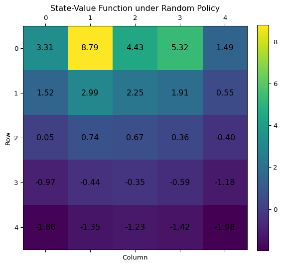

Figure 3.1: This is like the right part of Figure 3.2 (Sutton and Barto 2018): the state-value function for the equiprobable random policy

Exercise 3.14 The Bellman equation (Equation 3.12) must hold for each state for the value function $v_\pi$ shown in Figure 3.1 of Example 3.1. Show numerically that this equation holds for the center state, valued at +0.7, with respect to its four neighboring states, valued at +2.3, +0.4, 0.4, and +0.7. (These numbers are accurate only to one decimal place.)

Solution 3.14. We’ll use the numbers accurate to two decimal places. Basically we have to show that for the middle state $s$ we have \[ \begin{split} v_\pi(s) &\approx 0.9 \cdot 0.25 \cdot \big( v_\pi(s + (1,0)) + v_\pi(s + (-1,0)) \\ &+ v_\pi(s + (0,1)) + v_\pi(s + (0,-1)) \big), \end{split} \] (Here, we’re using vector notation to denote the directions to neighbouring states.)

Indeed this is true \[ 0.9 \cdot 0.25 \cdot (2.25 + 0.36 + (-0.35) + 0.74) = 0.669 \] which is approximately $0.67$

Exercise 3.15 In the gridworld example, rewards are positive for goals, negative for running into the edge of the world, and zero the rest of the time. Are the signs of these rewards important, or only the intervals between them? Prove, using Equation 3.3, that adding a constant $c$ to all the rewards adds a constant, $v_c$, to the values of all states, and thus does not affect the relative values of any states under any policies. What is $v_c$ in terms of $c$ and $\gamma$?

Solution 3.15. Adding a constant $c$ to all rewards in a continuing task adds a constant \[ v_c = \frac{c}{ 1 − \gamma} \] to the value of every state. This can be shown as follows. \[ \begin{split} G_t &= \sum_{k=0}^{\infty} \gamma^k (R_{t+k+1} + c) \\ &= \sum_{k=0}^{\infty} \gamma^k R_{t+k+1} + \sum_{k=0}^\infty \gamma^kc\\ &= \sum_{k=0}^{\infty} \gamma^k R_{t+k+1} + \frac{c}{1-\gamma} \end{split} \]

Thus, the relative ordering of state values is preserved (it doesn’t change which states are better than others). However, value ratios do change.

For completeness, we can also verify this result using the vector form of the Bellman equation. Suppose $\mathbf{v}$ is the original value function, and $\mathbf{r}$ the original reward vector. After adding a constant $c$ to every reward, the new reward vector is $r+c\mathbf{1}$, where $\mathbf{1}$ is the vector of all ones. The new value function is \[ \begin{split} \mathbf{v}' &= (\mathbf{I} - \gamma \mathbf{P})^{-1} (\mathbf{r} + c\mathbf{1}) \\ &= (\mathbf{I} - \gamma \mathbf{P})^{-1} \mathbf{r} + c(\mathbf{I} - \gamma \mathbf{P})^{-1} \mathbf{1} \\ &= \mathbf{v} + \frac{c}{1 - \gamma} \mathbf{1}, \end{split} \] since $(\mathbf{I} - \gamma \mathbf{P}) \frac{1}{1-\gamma}\mathbf{1} = \frac{1}{1-\gamma}(\mathbf{1} - \gamma \mathbf{1}) = \mathbf{1}$.

Exercise 3.16 Now consider adding a constant $c$ to all the rewards in an episodic task, such as maze running. Would this have any effect, or would it leave the task unchanged as in the continuing task above? Why or why not? Give an example.

Solution 3.16. In an episodic task, adding a constant $c$ to all rewards the task in a meaningful way. The additive term depends on both the state and the policy through the expected remaining time in the episode, so it can change the relative values of states and also reverse the ranking of policies.

Formally, for the undiscounted case, the value function under a modified reward $R'_t = R_t + c$ becomes:

\[ \begin{split} v'_{\pi}(s) &= \mathbb{E}_{\pi}\left[\sum_{k=0}^{T-t-1} (R_{t+k+1} + c) \mid S_t = s \right] \\ &= v_{\pi}(s) + c \cdot \mathbb{E}_{\pi}[T - t \mid S_t = s], \end{split} \] where $T$ is the random variable for the time step at which the episode ends.

We consider the easiest maze in the world with two states: $S$ and $T$ (terminal). In state $S$, there are two actions:

“continue”: returns to $S$ with reward $r$
“stop”: transitions to $T$ with reward $0$

If $r=−1$, then policies that choose “stop” with highen probability perform better. However, if we add $c=2$ to all rewards, then this reverses to selecting “stop” with lower probability.

Exercise 3.17 What is the Bellman equation for action values, that is, for $q_\pi$? It must give the action values $q_\pi(s,a)$ in terms of the action values $q_\pi(s'a')$, of possible successors to the state-action pair $(s,a)$.

Solution 3.17. This is just Equation 3.13.

Exercise 3.18 The value of a state depends on the values of the actions possible in that state and on how likely each action is to be taken under the current policy. We can think of this in terms of a small backup diagram rooted at the state and considering each possible action:

Give the equation corresponding to this intuition and diagram for the value at the root node, $v_\pi(s)$, in terms of the value at the expected leaf node, $q_{\pi}(s, a)$, given $S_t = s$. This equation should include an expectation conditioned on following the policy, $\pi$. Then give a second equation in which the expected value is written out xplicitly in terms of $\pi(a|s)$ such that no expected value notation appears in the equation.

Solution 3.18. The hardest part of this exercise is to understand the problem description. And in the end isn’t this just Exercise 3.12 again? \[ \begin{split} v_{\pi}(s) &= \mathbb{E}_{\pi}[q_\pi(s, A_t) \mid S_t = s] \\ &= \sum_{a} \pi(a|s)q_{\pi}(s,a) \end{split} \]

Exercise 3.19 The value of an action, $q_{\pi}(s, a)$, depends on the expected next reward and the expected sum of the remaining rewards. Again we can think of this in terms of a small backup diagram, this one rooted at an action (state–action pair) and branching to the possible next states:

Give the equation corresponding to this intuition and diagram for the action value, $q_{\pi}(s, a)$, in terms of the expected next reward, $R_{t+1}$, and the expected next state value, $v_{\pi}(S_{t+1})$, given that $S_{t} = s$

Solution 3.19. Ok, let’s do it again. \[ \begin{split} q_{\pi}(s,a) &= \mathbb{E}[R_{t+1} + \gamma v_{\pi}(S_{t+1}) \mid S_t = s, A_t = a] \\ &= \sum_{s',r} p(s',r|s,a) [r + \gamma v_{\pi}(s')] \end{split} \]

Note, I have left out the subscript $\pi$ for the expectation as the transition $(S_t,A_t)\to (S_{t+1}, R_{t+1})$ is independent of the agent.

3.6 Optimal Policies and Optimal Value Functions

In the next chapter (Section 4.2), we will see that any MDP has an optimal deterministic policy. We’ll take this fact for granted for now and focus on their value functions.

A policy is deterministic if $\pi(a|s) = 1$ for exactly one action for each $s \in \mathcal{S}$. We then also just write $\pi(s)$ for this action.

A policy $\pi_*$ is optimal if $\pi_* \geq \pi$ for any other $\pi$. Here we use $\geq$, a partial order on all policies for the MDP, defiend by \[ \pi \leq \pi' \quad:\Longleftrightarrow\quad v_\pi(s) \leq \pi'(s) \; \text{, for all }s \in \mathcal{S}. \]

There might be more than one optimal policy, but they must have the same value function (otherwise, they wouldn’t be optimal). We can define the optimal state-value function as \[ v_*(s) := \max_{\pi} v_{\pi}(s) \]

and the optimal action-value function as \[ q_*(s,a) := \max_{\pi} q_\pi(s,a). \]

These definitions are well-defined by the existence of optimal policies.

The conversion formula from $q_*$ to $v_*$ takes a special simple form (we also prove this in the next chapter in Theorem 4.2): \[ v_*(s) = \max_{a} q_\pi(a,s) \]

Combining this with Equation 3.9, we get the Bellman optimality equations for the state value: \[ v_*(s) = \max_{a} \sum_{s',r}p(s',r|s,a)[r + \gamma v_*(s')] \]

and the state-action value: \[ q_*(s,a) = \sum_{s',r}p(s',r|s,a) [r + \gamma \max_{a'}q_*(s',a')] \]

In principal, these Bellman optimality equations can be solved and having access to either $v_*$ or $q_*$ gives us direct access to an optimal $\pi_*$ (for $v_* \to \pi_*$ we need to know the dynamics of the MDP though; see Exercise 3.28)

Exercise 3.20 Draw or describe the optimal state-value function for the golf example.

Solution 3.20. I’m not 100% sure about this solution as I don’t like the golf example too much and as a result haven’t thought it completely through:

Use driver when not on the green. Use putter on the green.

Exercise 3.21 Draw or describe the contours of the optimal action-value function for putting, $q_*(s, \mathrm{putter})$, for the golf example.

Solution 3.21. I’m even less sure here.

Inside the -2 contour of $v_\mathrm{putt}$ it’s like $v_{\mathrm{putt}}$. In the sand it’s -3. Everywhere else it’s like the $q_*(s,\mathrm{driver})$ but shifted by a putter distance outwards and the value is one less.

Exercise 3.22 Consider the continuing MDP shown on to the right. The only decision to be made is that in the top state, where two actions are available, $\mathrm{left}$ and $\mathrm{right}$. The numbers show the rewards that are received deterministically after each action. There are exactly two deterministic policies, $\pi_{\mathrm{left}}$ and $\pi_{\mathrm{right}}$. What policy is optimal if $\gamma = 0$? If $\gamma = 0.9$? If $\gamma = 0.5$?

Solution 3.22. Here is a table indicating which policy is best in which case.

$\gamma$	$v_{\pi_{\mathrm{left}}}$	$v_{\pi_{\mathrm{right}}}$
0	1	0
0.9	1	1.8
0.5	0.5	0.5

Exercise 3.23 Give the Bellman equation for $q_*$ for the recycling robot.

Solution 3.23.

Exercise 3.24 Figure 3.5 gives the optimal value of the best state of the gridworld as 24.4, to one decimal place. Use your knowledge of the optimal policy and (3.8) to express this value symbolically, and then to compute it to three decimal places.

Solution 3.24. The solution is \[ \begin{split} v_*(s) &= 10 + 0\gamma + 0\gamma^2 + 0\gamma^3 + 0\gamma^4 + 10\gamma^5 + \dots \\ &= 10 \sum_{i=0}^\infty \gamma^{5i} = \frac{10}{1-\gamma^5} \end{split} \] Which is for $\gamma = 0.9$ approximately $24.41943$.

Exercise 3.25 Give an equation for $v_*$ in terms of $q_*$.

Solution 3.25. \[ v_*(s) = \max_a q_*(s,a) \]

Exercise 3.26 Give an equation for $q_*$ in terms of $v_*$ and the four-argument $p$.

Solution 3.26. \[ q_*(s,a) = \sum_{s',r} p(s',r|s,a) [r + \gamma v_*(s)] \]

Exercise 3.27 Give an equation for $\pi_*$ in terms of $q_\pi$.

Solution 3.27. \[ \pi_*(s) = \underset{a}{\mathrm{argmax}} \; q_*(s,a) \]

Exercise 3.28 Give an equation for $\pi_*$ in terms of $v_*$ and the four-argument $p$.

Solution 3.28. \[ \pi_*(s) = \underset{a}{\mathrm{argmax}} \sum_{s',r} p(s',r|s,a) [r + \gamma v_*(s)] \]

Exercise 3.29 Rewrite the four Bellman equations for the four value functions ($v_\pi$, $v_*$, $q_\pi$, and $q_*$) in terms of the three argument function $p$ (3.4) and the two-argument function $r$ (3.5).

Solution 3.29. \[ \begin{split} v_\pi(s) &= \sum_{a} \pi(a|s) \Big[r(a,s) + \gamma \sum_{s'} p(s'|a,s) v_\pi(s')\Big] \\ v_*(s) &= \max_a r(a,s) + \gamma \sum_{s'} p(s'|a,s) v_*(s') \\ q_\pi(a,s) &= r(a,s) + \gamma \sum_{s'} p(s'|s,a) \sum_{a'} \pi(a'|s') q_\pi(a',s') \\ q_*(a,s) &= r(a,s) + \gamma \sum_{s'} p(s'|s,a) \max_{a'} q_*(a',s') \end{split} \]

3.7 Optimality and Approximation

3.8 Summary

Sutton, Richard S., and Andrew G. Barto. 2018. Reinforcement Learning: An Introduction. Second edition. Adaptive Computation and Machine Learning Series. Cambridge, MA: MIT Press. https://mitpress.mit.edu/9780262039246/reinforcement-learning/.

“Our” Markov processes could be called more precisely stationary discrete-time Markov process.↩︎

t	\(R_{t+1}\)	\(\gamma G_{t+1}\)	\(G_t\)
5	0	0	0
4	2	0	2
3	3	1	4
2	6	2	8
1	2	8	10
0	1	5	6